
机器学习基础
发布时间:
This is a sample blog post.
机器学习
数据
xx
机器学习算法
监督学习/无监督学习/半监督学习/自监督学习等
线性模型
决策树
支持向量机
贝叶斯分类器
集成学习
无监督聚类
降维与度量学习
特征选择与稀疏学习
半监督学习
概率图模型
马尔科夫链
神经网络
强化学习
深度学习
参考教材:
- 2016年 南京大学周志华《机器学习》( 西瓜书)
- 2020年 复旦大学邱锡鹏 《神经网络与深度学习》(蒲公英书)https://nndl.github.io/
- 2023年 PumpkinBook(南瓜书)(旨在对西瓜书里比较难理解的公式加以解析,以及对部分公式补充具体的推导细节。)https://datawhalechina.github.io/pumpkin-book/#/
- 2017年麻省理工学院 Ian Goodfellow、Yoshua Bengio 和 Aaron Courville《深度学习》(花书)https://github.com/exacity/deeplearningbook-chinese; https://github.com/MingchaoZhu/DeepLearning
- 2023年(较新、前言)University of Bath 西蒙·普林斯/Simon J. D. Prince 《Understanding Deep Learning》 https://udlbook.github.io/udlbook/
- 2012年 李航《统计学习方法》 https://github.com/DefTruth/statistic-learning-R-note
数据
HF Curate high-quality datasets
神经网络模型
CNN
特点:局部感知、参数共享
- 卷积层
- 非线性激活函数
- 引入非线性激活函数的目的是提高神经网络的非线性拟合能力,增强模型的表达能力。
- sigmoid,tanh,relu。
- 激活函数,激活函数能为网络增加非线性使网络有更好的拟合能力
- 池化层
- 全连接层
- Dropout层
- 训练的过程中随机的将部分神经元的激活函数设置为0不参与计算,可以在训练的过程中产生不同的模型,不同的模型的输出不同,但是计算结果在同一个范围内波动,可以将最终结果看作这些模型的平均输出,减少神经元之间的依赖,提升泛化性能
- Dropout可以跟在全连接层后面、卷积层后面、注意力后面。
- 在全连接层中,Dropout层一般位于激活函数层之后。这样做的原因是,对于某些激活函数,如ReLU,当输入为0时,输出也为0,因此Dropout层的加入可能不会产生预期效果。不过,对于ReLU来说,由于输入0时输出也是0,所以放在激活函数后的问题不大。对于卷积层,由于参数较少,很少将Dropout层放在卷积层后面,卷积层通常使用BatchNorm层来正则化模型。
- BN层
- 将一个batch内的样本内的所有特征归一化为符合正态分布的数据(均值为0,方差为1),最后对归一化的数据进行缩放和偏移来还原数据本身的分布。
- BN,BN能够有效减小神经网络训练过程中产生的Internal Covariate Shift问题
- LN层:对每个样本的所有特征进行归一化。适用场景:LN适用于处理不定长行为序列场景,因为如果使用BN,padding的部分特征pooling会扰乱正常非padding的那部分特征。
- LayerNorm和BatchNorm:https://zhuanlan.zhihu.com/p/656647661
- BatchNorm是对一个特征维度做正则化,CNN中的LayerNorm是对一个样本做正则化,Transformer中的LayerNorm是对一个词(而不是一个句子)做正则化。
- BatchNorm(批归一化)层的位置可以有所不同,有的研究将其放在激活层之后,而有的则放在激活层之前。
class Mlp(nn.Module):
    """ Multilayer perceptron."""

    def __init__(self, in_features, hidden_features=None, out_features=None, act_layer=nn.GELU, drop=0.):
        super().__init__()
        out_features = out_features or in_features
        hidden_features = hidden_features or in_features
        self.fc1 = nn.Linear(in_features, hidden_features)
        self.act = act_layer()
        self.fc2 = nn.Linear(hidden_features, out_features)
        self.drop = nn.Dropout(drop)

    def forward(self, x):
        x = self.fc1(x)
        x = self.act(x)
        x = self.drop(x)
        x = self.fc2(x)
        x = self.drop(x)
        return x
"""resnet in pytorch


[1] Kaiming He, Xiangyu Zhang, Shaoqing Ren, Jian Sun.

    Deep Residual Learning for Image Recognition
    https://arxiv.org/abs/1512.03385v1
"""

import torch
import torch.nn as nn

class BasicBlock(nn.Module):
    """Basic Block for resnet 18 and resnet 34

    """

    #BasicBlock and BottleNeck block
    #have different output size
    #we use class attribute expansion
    #to distinct
    expansion = 1

    def __init__(self, in_channels, out_channels, stride=1):
        super().__init__()

        #residual function
        self.residual_function = nn.Sequential(
            nn.Conv2d(in_channels, out_channels, kernel_size=3, stride=stride, padding=1, bias=False),
            nn.BatchNorm2d(out_channels),
            nn.ReLU(inplace=True),
            nn.Conv2d(out_channels, out_channels * BasicBlock.expansion, kernel_size=3, padding=1, bias=False),
            nn.BatchNorm2d(out_channels * BasicBlock.expansion)
        )

        #shortcut
        self.shortcut = nn.Sequential()

        #the shortcut output dimension is not the same with residual function
        #use 1*1 convolution to match the dimension
        if stride != 1 or in_channels != BasicBlock.expansion * out_channels:
            self.shortcut = nn.Sequential(
                nn.Conv2d(in_channels, out_channels * BasicBlock.expansion, kernel_size=1, stride=stride, bias=False),
                nn.BatchNorm2d(out_channels * BasicBlock.expansion)
            )

    def forward(self, x):
        return nn.ReLU(inplace=True)(self.residual_function(x) + self.shortcut(x))

class BottleNeck(nn.Module):
    """Residual block for resnet over 50 layers

    """
    expansion = 4
    def __init__(self, in_channels, out_channels, stride=1):
        super().__init__()
        self.residual_function = nn.Sequential(
            nn.Conv2d(in_channels, out_channels, kernel_size=1, bias=False),
            nn.BatchNorm2d(out_channels),
            nn.ReLU(inplace=True),
            nn.Conv2d(out_channels, out_channels, stride=stride, kernel_size=3, padding=1, bias=False),
            nn.BatchNorm2d(out_channels),
            nn.ReLU(inplace=True),
            nn.Conv2d(out_channels, out_channels * BottleNeck.expansion, kernel_size=1, bias=False),
            nn.BatchNorm2d(out_channels * BottleNeck.expansion),
        )

        self.shortcut = nn.Sequential()

        if stride != 1 or in_channels != out_channels * BottleNeck.expansion:
            self.shortcut = nn.Sequential(
                nn.Conv2d(in_channels, out_channels * BottleNeck.expansion, stride=stride, kernel_size=1, bias=False),
                nn.BatchNorm2d(out_channels * BottleNeck.expansion)
            )

    def forward(self, x):
        return nn.ReLU(inplace=True)(self.residual_function(x) + self.shortcut(x))

class ResNet(nn.Module):

    def __init__(self, block, num_block, num_classes=100):
        super().__init__()

        self.in_channels = 64

        self.conv1 = nn.Sequential(
            nn.Conv2d(3, 64, kernel_size=3, padding=1, bias=False),
            nn.BatchNorm2d(64),
            nn.ReLU(inplace=True))
        #we use a different inputsize than the original paper
        #so conv2_x's stride is 1
        self.conv2_x = self._make_layer(block, 64, num_block[0], 1)
        self.conv3_x = self._make_layer(block, 128, num_block[1], 2)
        self.conv4_x = self._make_layer(block, 256, num_block[2], 2)
        self.conv5_x = self._make_layer(block, 512, num_block[3], 2)
        self.avg_pool = nn.AdaptiveAvgPool2d((1, 1))
        self.fc = nn.Linear(512 * block.expansion, num_classes)

    def _make_layer(self, block, out_channels, num_blocks, stride):
        """make resnet layers(by layer i didnt mean this 'layer' was the
        same as a neuron netowork layer, ex. conv layer), one layer may
        contain more than one residual block

        Args:
            block: block type, basic block or bottle neck block
            out_channels: output depth channel number of this layer
            num_blocks: how many blocks per layer
            stride: the stride of the first block of this layer

        Return:
            return a resnet layer
        """

        # we have num_block blocks per layer, the first block
        # could be 1 or 2, other blocks would always be 1
        strides = [stride] + [1] * (num_blocks - 1)
        layers = []
        for stride in strides:
            layers.append(block(self.in_channels, out_channels, stride))
            self.in_channels = out_channels * block.expansion

        return nn.Sequential(*layers)

    def forward(self, x):
        output = self.conv1(x)
        output = self.conv2_x(output)
        output = self.conv3_x(output)
        output = self.conv4_x(output)
        output = self.conv5_x(output)
        output = self.avg_pool(output)
        output = output.view(output.size(0), -1)
        output = self.fc(output)

        return output

def resnet18():
    """ return a ResNet 18 object
    """
    return ResNet(BasicBlock, [2, 2, 2, 2])

def resnet34():
    """ return a ResNet 34 object
    """
    return ResNet(BasicBlock, [3, 4, 6, 3])

def resnet50():
    """ return a ResNet 50 object
    """
    return ResNet(BottleNeck, [3, 4, 6, 3])

def resnet101():
    """ return a ResNet 101 object
    """
    return ResNet(BottleNeck, [3, 4, 23, 3])

def resnet152():
    """ return a ResNet 152 object
    """
    return ResNet(BottleNeck, [3, 8, 36, 3])
RNN
- LSTM
- GRU
- …
Transformer
NLP:Bert、GPT
Vision:ViT、ViViT
常见任务
NLP任务
NLP主要分为两大类任务NLU(自然语言理解)和NLG(自然语言生成)。
| Model | Examples | Tasks |
|---|---|---|
| Encoder-only | BERT, DistilBERT, ModernBERT | Sentence classification, named entity recognition, extractive question answering |
| Decoder-only | GPT, LLaMA, Gemma, SmolLM | Text generation, conversational AI, creative writing |
| Encoder-decoder | BART, T5, Marian, mBART | Summarization, translation, generative question answering |
视觉任务
HF Community Computer Vision Course
| Feature | Image | Video | |
|---|---|---|---|
| 1 | Type | Single moment in time | Sequence of images over time |
| 2 | Data Representation | Typically a 2D array of pixels | Typically a 3D array of frames |
| 3 | File types | JPEG,PNG,RAW, etc. | MP4,AVI, MOV, etc. |
| 4 | Data Augmentation | Flipping, rotating, cropping | Temporal jittering, speed variations, occlusion |
| 5 | Feature Extraction | Edges, textures, colors | Edges, textures, colors, optical flow, trajectories |
| 6 | Learning Models | CNNs | RNNs, 3D CNNs |
| 7 | Machine Learning Tasks | Image classification, Segmentation, Object Detection | Video action recognition, temporal modeling, tracking |
| 8 | Computational Cost | Less expensive | More expensive |
| 9 | Applications | Facial recognition for security access control | Sign language interpretation for live communication |
模型训练
# Hugging Face gives a complete training loop with 🤗 Accelerate in https://huggingface.co/learn/llm-course/chapter3/4

from accelerate import Accelerator
from torch.optim import AdamW
from transformers import AutoModelForSequenceClassification, get_scheduler

accelerator = Accelerator()

model = AutoModelForSequenceClassification.from_pretrained(checkpoint, num_labels=2)
optimizer = AdamW(model.parameters(), lr=3e-5)

train_dl, eval_dl, model, optimizer = accelerator.prepare(
    train_dataloader, eval_dataloader, model, optimizer
)

num_epochs = 3
num_training_steps = num_epochs * len(train_dl)
lr_scheduler = get_scheduler(
    "linear",
    optimizer=optimizer,
    num_warmup_steps=0,
    num_training_steps=num_training_steps,
)

progress_bar = tqdm(range(num_training_steps))

model.train()
for epoch in range(num_epochs):
    for batch in train_dl:
        outputs = model(**batch)
        loss = outputs.loss
        accelerator.backward(loss)

        optimizer.step()
        lr_scheduler.step()
        optimizer.zero_grad()
        progress_bar.update(1)
数据准备
数据集构建 Dataset
数据预处理
数据筛选
数据增强
数据归一化(Normalization)
数据集加载 DataLoader
Loss
分类Loss
信息量
信息奠基人香农(Shannon)认为“信息是用来消除随机不确定性的东西”,也就是说衡量信息量的大小就是看这个信息消除不确定性的程度。信息量的大小与信息发生的概率成反比。概率越大,信息量越小。概率越小,信息量越大。设某一事件发生的概率P(x),其信息量表示为: \(I(x) = -logp(x)\)
信息熵
信息熵也被称为熵,用来表示所有信息量的期望。 \(H ( X ) = - \sum _ { i = 1 } ^ { n } P ( x _ { i } ) \log ( P ( x _ { i } ) ) ,X = ( x _ { 1 } , x _ { 2 } , \ldots , x _ { n } )\)
KL散度
KL散度用来衡量两个概率分布之间的相似度。 \(D_{KL}(P||Q)=\sum_{i=1}^{n}P(x_{i})\frac{log(P(x_{i}))}{log(Q(x_{i})}\\ P(x_{i})表示真实概率分布、Q(x_{i})表示预测概率分布,\\Q(x_{i})越接近P(x_{i}),KL散度越小。\)
交叉熵
KL散度拆开形似为: \(D_{KL}(P||Q)=\sum_{i=1}^{n}P(x_{i})\frac{log(P(x_{i}))}{log(Q(x_{i})}\\=\sum_{i=1}^{n}P(x_{i})\log(P(x_{i}))-\sum_{i=1}^{n}P(x_{i})\log(Q(x_{i}))\\ \sum_{i=1}^{n}P(x_{i})\log(P(x_{i}))为信息熵;\\ \sum_{i=1}^{n}P(x_{i})\log(Q(x_{i}))为交叉熵;\\\) 由于信息熵不变,所以交叉熵越小,预测概率的分布和原始分布越接近, 所以优化的时候按交叉熵来优化即可。
求导 \(分类问题中,P(x_{i})为目标one-hot形似的标签,这里用y_{i}表示,Q(x_{i})为\\softmax函数的输出用a_{i}表示,交叉熵形式为\\ L=-\sum_{j}y_{i}lna_{j}\\ a_{i} = \frac{e^{z^i}}{\sum_{k}e^{z^k}}\)
\[\left\{\begin{array}{ll} \frac{dL}{dz^i}=\frac{d(-\sum_{j}y_{i}lna_{j})}{da_{j}}.\frac{da_{j}}{dz^i}=-\frac{dL}{da_{j}}.\frac{da_{j}}{dz^i}\\ =-\sum_{j}\frac{y_{j}}{a_{j}}.\frac{da_{j}}{dz_{j}}\\ =-(\sum_{i=j}\frac{y_{i}}{a_{i}}.\frac{da_{i}}{dz_{i}}+\sum_{i!=j}\frac{y_{j}}{a_{j}}.\frac{da_{j}}{dz_{i}})\\ \frac{da_{i}}{dz_{i}}=a_{i}.(1-a_{i}),i==j\\ \frac{da_{j}}{dz_{i}}=-a_{j}.a_{i},i!=j\\ \frac{dL}{dz^i}=a_{i}.\sum_{j}y_{j}-y_{i}\\ 因为y_{i}是one-hot标签,所以\frac{dL}{dz^i}=a_{i}-y_{i} \end{array}\right.\]
交叉熵损失,是分类任务中最常用的一个损失函数。在Pytorch中是基于下面的公式实现的。
\(\operatorname{Loss}(\hat{x}, x)=-\sum_{i=1}^{n} x \log (\hat{x})\) 其中 $x$ 是真实标签, $\hat{x}$ 是预测的类分布(通常是使用softmax将模型输出转换为概率分布)。
取单个样本举例, 假设 $x_{1}$=[0, 1, 0],模型预测样本的概率$\hat{x_{1}}$为 [ 0.1 , 0.5 , 0.4 ]。则样本的损失计算如下所示: \(\operatorname{Loss}\left(\hat{x_{1}}, x_{1}\right)=-0 \times \log (0.1)-1 \times \log (0.5)-0 \times \log (0.4)=\log (0.5)\) 实际使用中需要注意几点:
- torch.nn.CrossEntropyLoss(input, target)中的标签target使用的不是one-hot形式,而是类别的序号。形如 target = [0, 2, 1] 表示3个样本分别属于第1类、第3类、第2类。(单标签多分类问题)
- torch.nn.CrossEntropyLoss(input, target)的input是没有归一化的每个类的得分,而不是softmax之后的分布。
import torch
loss_func = torch.nn.CrossEntropyLoss()

input = torch.tensor([[0.13, -0.18, 0.87],
		 [0.25, -0.04, 0.32],
		 [0.24, -0.54, 0.53]])
target = torch.tensor([0, 2, 1])

loss = loss_func(input, target)
Focal-loss
Focal-Loss可以在一定程度上降低样本类别不均衡带来的精度损失,通过简单easy-sample的loss值,提升hard-sample的loss值(相对提升)来促使网络更加关注难例。
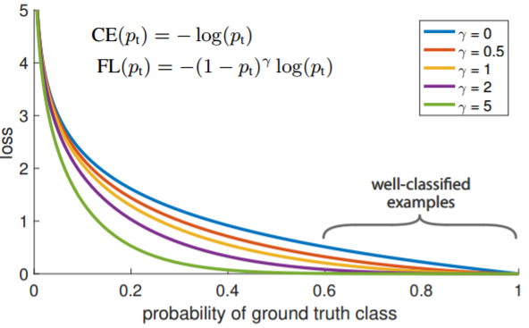
公式如下式所示: \(\large \mathrm{L}_{f l}= \begin{cases}-\alpha\left(1-y^{\prime}\right)^{\gamma} \log y^{\prime} \quad, & y=1 \\ -(1-\alpha) y^{\prime \gamma} \log \left(1-y^{\prime}\right), & y=0\end{cases}\\ \large 从上公式可以看出,focal-loss是从BCEloss的基础上添加了两部分:\gamma和\alpha,以y=1为例,当y^{\prime}越大时认为该样本比较容易学习就降低\\ \large 该样本的loss值,当y^{\prime}越小时就认为该样本越难学习就相对增加该样的权重(就是减小的少了)。\)
回归Loss
MSE损失
L1 Loss \(\large L_{L1}=\sum_{i=0}^{n}\left|y_{i}-y_{i}^{p}\right| / n\)
优点
不论对于什么样的输入值,都有着稳定的梯度,不会导致梯度爆炸问题,对离群点不敏感,具有较为稳健性的解。
缺点
在中心点是折点,不能求导,不方便求解。其导数为常数,导致训练后期,预测值与真是差异很小时,损失函数的导数绝对值仍然为1,而如果learning rate不变,损失函数将在稳定值附近波动,难以继续收敛达到更高精度
L2 Loss
公式 \(\large L_{L2}=\sum_{i=0}^{n}\left|y_{i}-y_{i}^{p}\right|^2 / n\)
优点
各点都连续光滑,方便求导,而且梯度值也是动态变化的,能够快速的收敛,得到较为稳定的解
缺点
真实值和预测值的差值大于1时,会放大误差;而当差值小于1时,则会缩小误差,这是平方运算决定的。MSE对于较大的误差>1给予较大的惩罚,较小的误差<1给予较小的惩罚。也就是说,对离群点比较敏感,受其影响较大。所以训练初期,一旦出现预测值和真实值差异很大时,就很容易出现梯度爆炸。
SmoothL1 Loss
公式 \(\large S m o o t h_{L 1}(x)=\left\{\begin{array}{ll} 0.5 x^{2} & \text { if }|x|<1 ; \\ \large |x|-0.5 & \text { else. } \large \end{array} \quad x=y_{i}-y_{i}^{p}\right.\)
优点
综合了L1和L2的优点,相比于L2损失函数,对离群点、异常值使用L1,梯度变化相对更小,训练时不容易跑飞。当预测值与真是差异很小时,使用L2损失,快速得到较为稳定的解。
缺点
L1,L2 loss也有相同缺点,就是他们都是分别回归宽高和中心点,没有把box当成一个整体看待。
IOU Loss
公式
优点
如下图所示,L1 和 L2 的边界框 L1 和 L2 loss 是相同的,但是他们的 IOU 却相差很大:
如果宽高和中心点使用分别优化的话就会损失他们之间的相关性,实际上目标回归框之间存在相关性,并不是相互独立的,使用 IOU LOSS可以把回归框当成一个整体去优化,如上图最右边的回归情况最好,最左边的回归情况最差,但是它们的 LS Loss 确实相同的,所以不合理。
缺点
- 预测值和 gt 不重叠,iou 始终为 0 且无法优化
- IOU 无法辨别不同的对其方式,如下图所示,下图三个的iou都是一样的
优化器optimazer
优化器在DL中起着灯塔的作用,指引参数往正确的方向更新,一个好的优化器能够使模型收敛速度加快,跳出局部最优,训练过程平稳等
梯度下降法:将损失函数作为目标函数,通过梯度下降法不断来调整模型参数,以最小化损失函数。 梯度下降法基本步骤: 1、选择初始参数值:网络参数随机初始化(一般比较小) 2、计算目标函数关于参数的梯度(梯度是目标函数在每个参数维度上的偏导数。梯度向量表示了函数值增长最快的方向) 3、更新参数:沿着梯度的反方向,以一定的学习率调整参数。学习率决定了每次参数更新的步长。(一般初期设置较大的学习率加速网络收敛,大的学习率可能导致在最优解附近震荡,当迭代次数增多,学习率逐渐减小,以保证收敛至全局最优解) 4、迭代:重复步骤2和3,直到满足停止条件,如达到一定的迭代次数,梯度接近零,或者函数值变化较小。 5、输出结果:最终参数值即为函数的极小值点。
- BGD:对所有样本更新一次参数,陷入局部最优+内存爆炸
- SGD,每个样本都更新一次参数,步长固定,很容易停滞在局部最小值;更新频繁,参数收敛过程震荡;
- Mini-batch GD:折中方法,每个batch更新一次参数,降低参数更新时的方差,相对于SGD更稳定,缺点是学习率的选择问题,需要先设置大一点再设置小一点。
- AdaGrad自适应学习率+动量加快速度:消除手动调整学习率的过程,根据迭代次数和累积梯度,使得刚开始迭代时,学习率较大,可以快速收敛。而后来则逐渐减小,模型可以稳定找到最优点。缺点是没有考虑迭代衰减,极端情况如果刚开始的梯度特别大,而后面的比较小,则学习率基本不会变化了。
- Adam优化器:自适应学习率+考虑迭代衰减(梯度求和时候加入衰减因子)+动量加快优化速度
目前我们还是主要以adgrad+动量为主,因为adam在实际应用中迭代速度过快容易陷入局部最优。
大模型时代,通常使用AdamW作为训练Transformer的优化器。
优化器,优化器就像灯塔指引网络往正确的方向收敛,一个好的优化器能够帮助网络快速收敛,跳出局部最优,训练过程更加稳定
学习率调度器
反向传播
参考教材:神经网络与深度学习nndl的4.4 反向传播算法和4.5自动梯度计算。
模型训练过程中常遇到的问题及解决方法:
- 过拟合、欠拟合:
- Understanding Learning Curves
- 正则项,加入正则项能有效避免模型过拟合同时使模型更加稀疏
- 对损失函数增加惩罚项,常用的惩罚项L1正则和L2正则。
- L1正则是权重w的绝对值之和,网络中的权重w会尽可能取0,实现参数稀疏化,也相当于减少了网络复杂度,防止过拟合。也可以用于特征选择
- L2正则是各个权重w平方和,网络中的权重w更接近0但不会取0,减小了网络参数复杂度,防止过拟合。
梯度爆炸、梯度消失
残差网络解决梯度消失问题
归一化解决梯度爆炸问题