
Hugging Face LLM Course
发布时间:
This is a blog post of hugging face LLM course summary.
Hugging Face LLM Course
- Hugging Face LLM Course
- Chapter 0. Setup
- Chapter 1. Transformer models
- 1. Introduction
- 2. Natural Language Processing and Large Language Models
- 3. Transformers, what can they do?
- Transformers are everywhere!
- Working with pipelines
- Available pipelines for different modalities
- Zero-shot classification
- Text generation
- Using any model from the Hub in a pipeline
- Mask filling
- Named entity recognition
- Question answering
- Summarization
- Translation
- Image and audio pipelines
- Combining data from multiple sources
- Conclusion
- 4. How do Transformers work?
- 5. How 🤗 Transformers solve tasks
- 6. Transformer Architectures
- 8. Deep dive into Text Generation Inference with LLMs
- 9. Bias and limitations
- 10. Summary
- Chapter 2. Using 🤗 Transformers
- Chapter 3. Fine-tuning a pretrained model
- Chapter 4. Sharing models and tokenizers
- Chapter 5. The 🤗 Datasets library
- Chapter 6. The 🤗 Tokenizers library
- 1. Introduction
- 2. Training a new tokenizer from an old one
- 3a. Fast tokenizers’ special powers
- 3b. Fast tokenizers in the QA pipeline
- 4. Normalization and pre-tokenization
- 5. Byte-Pair Encoding tokenization
- 6. WordPiece tokenization
- 7. Unigram tokenization
- 8. Building a tokenizer, block by block
- 9. Tokenizers, check!
- Chapter 7. Classical NLP tasks
- Chapter 8. How to ask for help
- Chapter 9. Building and sharing demos
- Chapter 10. Curate high-quality datasets
- Chapter 11. Fine-tune Large Language Models
- Chapter 12. Build Reasoning Models
课程链接:Hugging Face - LLM Couese
Chapter 0. Setup
1. Introduction
Welcome to the Hugging Face course! This introduction will guide you through setting up a working environment. If you’re just starting the course, we recommend you first take a look at Chapter 1, then come back and set up your environment so you can try the code yourself.
All the libraries that we’ll be using in this course are available as Python packages, so here we’ll show you how to set up a Python environment and install the specific libraries you’ll need.
We’ll cover two ways of setting up your working environment, using a Colab notebook or a Python virtual environment. Feel free to choose the one that resonates with you the most. For beginners, we strongly recommend that you get started by using a Colab notebook.
Note that we will not be covering the Windows system. If you’re running on Windows, we recommend following along using a Colab notebook. If you’re using a Linux distribution or macOS, you can use either approach described here.
Most of the course relies on you having a Hugging Face account. We recommend creating one now: create an account.
Using a Google Colab notebook
Using a Colab notebook is the simplest possible setup; boot up a notebook in your browser and get straight to coding!
If you’re not familiar with Colab, we recommend you start by following the introduction. Colab allows you to use some accelerating hardware, like GPUs or TPUs, and it is free for smaller workloads.
Once you’re comfortable moving around in Colab, create a new notebook and get started with the setup:

The next step is to install the libraries that we’ll be using in this course. We’ll use pip for the installation, which is the package manager for Python. In notebooks, you can run system commands by preceding them with the ! character, so you can install the 🤗 Transformers library as follows:
!pip install transformers
You can make sure the package was correctly installed by importing it within your Python runtime:
import transformers
This installs a very light version of 🤗 Transformers. In particular, no specific machine learning frameworks (like PyTorch or TensorFlow) are installed. Since we’ll be using a lot of different features of the library, we recommend installing the development version, which comes with all the required dependencies for pretty much any imaginable use case:
!pip install transformers[sentencepiece]
This will take a bit of time, but then you’ll be ready to go for the rest of the course!
Using a Python virtual environment
If you prefer to use a Python virtual environment, the first step is to install Python on your system. We recommend following this guide to get started.
Once you have Python installed, you should be able to run Python commands in your terminal. You can start by running the following command to ensure that it is correctly installed before proceeding to the next steps: python --version. This should print out the Python version now available on your system.
When running a Python command in your terminal, such as python --version, you should think of the program running your command as the “main” Python on your system. We recommend keeping this main installation free of any packages, and using it to create separate environments for each application you work on — this way, each application can have its own dependencies and packages, and you won’t need to worry about potential compatibility issues with other applications.
In Python this is done with virtual environments, which are self-contained directory trees that each contain a Python installation with a particular Python version alongside all the packages the application needs. Creating such a virtual environment can be done with a number of different tools, but we’ll use the official Python package for that purpose, which is called venv.
First, create the directory you’d like your application to live in — for example, you might want to make a new directory called transformers-course at the root of your home directory:
mkdir ~/transformers-course
cd ~/transformers-course
From inside this directory, create a virtual environment using the Python venv module:
python -m venv .env
You should now have a directory called .env in your otherwise empty folder:
ls -a
. .. .env
You can jump in and out of your virtual environment with the activate and deactivate scripts:
# Activate the virtual environment
source .env/bin/activate

# Deactivate the virtual environment
deactivate
You can make sure that the environment is activated by running the which python command: if it points to the virtual environment, then you have successfully activated it!
which python
/home/<user>/transformers-course/.env/bin/python
Installing dependencies
As in the previous section on using Google Colab instances, you’ll now need to install the packages required to continue. Again, you can install the development version of 🤗 Transformers using the pip package manager:
pip install "transformers[sentencepiece]"
You’re now all set up and ready to go!
Chapter 1. Transformer models
1. Introduction
Welcome to the 🤗 Course!
This course will teach you about large language models (LLMs) and natural language processing (NLP) using libraries from the Hugging Face ecosystem — 🤗 Transformers, 🤗 Datasets, 🤗 Tokenizers, and 🤗 Accelerate — as well as the Hugging Face Hub.
We’ll also cover libraries outside the Hugging Face ecosystem. These are amazing contributions to the AI community and incredibly useful tools.
It’s completely free and without ads.
Understanding NLP and LLMs
While this course was originally focused on NLP (Natural Language Processing), it has evolved to emphasize Large Language Models (LLMs), which represent the latest advancement in the field.
What’s the difference?
- NLP (Natural Language Processing) is the broader field focused on enabling computers to understand, interpret, and generate human language. NLP encompasses many techniques and tasks such as sentiment analysis, named entity recognition, and machine translation.
- LLMs (Large Language Models) are a powerful subset of NLP models characterized by their massive size, extensive training data, and ability to perform a wide range of language tasks with minimal task-specific training. Models like the Llama, GPT, or Claude series are examples of LLMs that have revolutionized what’s possible in NLP.
Throughout this course, you’ll learn about both traditional NLP concepts and cutting-edge LLM techniques, as understanding the foundations of NLP is crucial for working effectively with LLMs.
What to expect?
Here is a brief overview of the course:

- Chapters 1 to 4 provide an introduction to the main concepts of the 🤗 Transformers library. By the end of this part of the course, you will be familiar with how Transformer models work and will know how to use a model from the Hugging Face Hub, fine-tune it on a dataset, and share your results on the Hub!
- Chapters 5 to 8 teach the basics of 🤗 Datasets and 🤗 Tokenizers before diving into classic NLP tasks and LLM techniques. By the end of this part, you will be able to tackle the most common language processing challenges by yourself.
- Chapter 9 goes beyond NLP to cover how to build and share demos of your models on the 🤗 Hub. By the end of this part, you will be ready to showcase your 🤗 Transformers application to the world!
- Chapters 10 to 12 dive into advanced LLM topics like fine-tuning, curating high-quality datasets, and building reasoning models.
This course:
- Requires a good knowledge of Python
- Is better taken after an introductory deep learning course, such as fast.ai’s Practical Deep Learning for Coders or one of the programs developed by DeepLearning.AI
- Does not expect prior PyTorch or TensorFlow knowledge, though some familiarity with either of those will help
After you’ve completed this course, we recommend checking out DeepLearning.AI’s Natural Language Processing Specialization, which covers a wide range of traditional NLP models like naive Bayes and LSTMs that are well worth knowing about!
Who are we?
About the authors:
Abubakar Abid completed his PhD at Stanford in applied machine learning. During his PhD, he founded Gradio, an open-source Python library that has been used to build over 600,000 machine learning demos. Gradio was acquired by Hugging Face, which is where Abubakar now serves as a machine learning team lead.
Ben Burtenshaw is a Machine Learning Engineer at Hugging Face. He completed his PhD in Natural Language Processing at the University of Antwerp, where he applied Transformer models to generate children stories for the purpose of improving literacy skills. Since then, he has focused on educational materials and tools for the wider community.
Matthew Carrigan is a Machine Learning Engineer at Hugging Face. He lives in Dublin, Ireland and previously worked as an ML engineer at Parse.ly and before that as a post-doctoral researcher at Trinity College Dublin. He does not believe we’re going to get to AGI by scaling existing architectures, but has high hopes for robot immortality regardless.
Lysandre Debut is a Machine Learning Engineer at Hugging Face and has been working on the 🤗 Transformers library since the very early development stages. His aim is to make NLP accessible for everyone by developing tools with a very simple API.
Sylvain Gugger is a Research Engineer at Hugging Face and one of the core maintainers of the 🤗 Transformers library. Previously he was a Research Scientist at fast.ai, and he co-wrote Deep Learning for Coders with fastai and PyTorch with Jeremy Howard. The main focus of his research is on making deep learning more accessible, by designing and improving techniques that allow models to train fast on limited resources.
Dawood Khan is a Machine Learning Engineer at Hugging Face. He’s from NYC and graduated from New York University studying Computer Science. After working as an iOS Engineer for a few years, Dawood quit to start Gradio with his fellow co-founders. Gradio was eventually acquired by Hugging Face.
Merve Noyan is a developer advocate at Hugging Face, working on developing tools and building content around them to democratize machine learning for everyone.
Lucile Saulnier is a machine learning engineer at Hugging Face, developing and supporting the use of open source tools. She is also actively involved in many research projects in the field of Natural Language Processing such as collaborative training and BigScience.
Lewis Tunstall is a machine learning engineer at Hugging Face, focused on developing open-source tools and making them accessible to the wider community. He is also a co-author of the O’Reilly book Natural Language Processing with Transformers.
Leandro von Werra is a machine learning engineer in the open-source team at Hugging Face and also a co-author of the O’Reilly book Natural Language Processing with Transformers. He has several years of industry experience bringing NLP projects to production by working across the whole machine learning stack..
FAQ
Here are some answers to frequently asked questions:
Does taking this course lead to a certification? Currently we do not have any certification for this course. However, we are working on a certification program for the Hugging Face ecosystem – stay tuned!
How much time should I spend on this course? Each chapter in this course is designed to be completed in 1 week, with approximately 6-8 hours of work per week. However, you can take as much time as you need to complete the course.
Where can I ask a question if I have one? If you have a question about any section of the course, just click on the “Ask a question” banner at the top of the page to be automatically redirected to the right section of the Hugging Face forums:
Note that a list of project ideas is also available on the forums if you wish to practice more once you have completed the course.
- Where can I get the code for the course? For each section, click on the banner at the top of the page to run the code in either Google Colab or Amazon SageMaker Studio Lab:
The Jupyter notebooks containing all the code from the course are hosted on the huggingface/notebooks repo. If you wish to generate them locally, check out the instructions in the course repo on GitHub.
How can I contribute to the course? There are many ways to contribute to the course! If you find a typo or a bug, please open an issue on the
courserepo. If you would like to help translate the course into your native language, check out the instructions here.What were the choices made for each translation? Each translation has a glossary and
TRANSLATING.txtfile that details the choices that were made for machine learning jargon etc. You can find an example for German here.Can I reuse this course? Of course! The course is released under the permissive Apache 2 license. This means that you must give appropriate credit, provide a link to the license, and indicate if changes were made. You may do so in any reasonable manner, but not in any way that suggests the licensor endorses you or your use. If you would like to cite the course, please use the following BibTeX:
@misc{huggingfacecourse,
  author = {Hugging Face},
  title = {The Hugging Face Course, 2022},
  howpublished = "\url{https://huggingface.co/course}",
  year = {2022},
  note = "[Online; accessed <today>]"
}
Languages and translations
Thanks to our wonderful community, the course is available in many languages beyond English 🔥! Check out the table below to see which languages are available and who contributed to the translations:
| Language | Authors |
|---|---|
| French | @lbourdois, @ChainYo, @melaniedrevet, @abdouaziz |
| Vietnamese | @honghanhh |
| Chinese (simplified) | @zhlhyx, petrichor1122, @yaoqih |
| Bengali (WIP) | @avishek-018, @eNipu |
| German (WIP) | @JesperDramsch, @MarcusFra, @fabridamicelli |
| Spanish (WIP) | @camartinezbu, @munozariasjm, @fordaz |
| Persian (WIP) | @jowharshamshiri, @schoobani |
| Gujarati (WIP) | @pandyaved98 |
| Hebrew (WIP) | @omer-dor |
| Hindi (WIP) | @pandyaved98 |
| Bahasa Indonesia (WIP) | @gstdl |
| Italian (WIP) | @CaterinaBi, @ClonedOne, @Nolanogenn, @EdAbati, @gdacciaro |
| Japanese (WIP) | @hiromu166, @younesbelkada, @HiromuHota |
| Korean (WIP) | @Doohae, @wonhyeongseo, @dlfrnaos19 |
| Portuguese (WIP) | @johnnv1, @victorescosta, @LincolnVS |
| Russian (WIP) | @pdumin, @svv73 |
| Thai (WIP) | @peeraponw, @a-krirk, @jomariya23156, @ckingkan |
| Turkish (WIP) | @tanersekmen, @mertbozkir, @ftarlaci, @akkasayaz |
| Chinese (traditional) (WIP) | @davidpeng86 |
For some languages, the course YouTube videos have subtitles in the language. You can enable them by first clicking the CC button in the bottom right corner of the video. Then, under the settings icon ⚙️, you can select the language you want by selecting the Subtitles/CC option.

[!TIP] Don’t see your language in the above table or you’d like to contribute to an existing translation? You can help us translate the course by following the instructions here.
Let’s go 🚀
Are you ready to roll? In this chapter, you will learn:
- How to use the
pipeline()function to solve NLP tasks such as text generation and classification - About the Transformer architecture
- How to distinguish between encoder, decoder, and encoder-decoder architectures and use cases
2. Natural Language Processing and Large Language Models
Before jumping into Transformer models, let’s do a quick overview of what natural language processing is, how large language models have transformed the field, and why we care about it.
What is NLP?
NLP is a field of linguistics and machine learning focused on understanding everything related to human language. The aim of NLP tasks is not only to understand single words individually, but to be able to understand the context of those words.
The following is a list of common NLP tasks, with some examples of each:
- Classifying whole sentences: Getting the sentiment of a review, detecting if an email is spam, determining if a sentence is grammatically correct or whether two sentences are logically related or not
- Classifying each word in a sentence: Identifying the grammatical components of a sentence (noun, verb, adjective), or the named entities (person, location, organization)
- Generating text content: Completing a prompt with auto-generated text, filling in the blanks in a text with masked words
- Extracting an answer from a text: Given a question and a context, extracting the answer to the question based on the information provided in the context
- Generating a new sentence from an input text: Translating a text into another language, summarizing a text
NLP isn’t limited to written text though. It also tackles complex challenges in speech recognition and computer vision, such as generating a transcript of an audio sample or a description of an image.
The Rise of Large Language Models (LLMs)
In recent years, the field of NLP has been revolutionized by Large Language Models (LLMs). These models, which include architectures like GPT (Generative Pre-trained Transformer) and Llama, have transformed what’s possible in language processing.
[!TIP] A large language model (LLM) is an AI model trained on massive amounts of text data that can understand and generate human-like text, recognize patterns in language, and perform a wide variety of language tasks without task-specific training. They represent a significant advancement in the field of natural language processing (NLP).
LLMs are characterized by:
- Scale: They contain millions, billions, or even hundreds of billions of parameters
- General capabilities: They can perform multiple tasks without task-specific training
- In-context learning: They can learn from examples provided in the prompt
- Emergent abilities: As these models grow in size, they demonstrate capabilities that weren’t explicitly programmed or anticipated
The advent of LLMs has shifted the paradigm from building specialized models for specific NLP tasks to using a single, large model that can be prompted or fine-tuned to address a wide range of language tasks. This has made sophisticated language processing more accessible while also introducing new challenges in areas like efficiency, ethics, and deployment.
However, LLMs also have important limitations:
- Hallucinations: They can generate incorrect information confidently
- Lack of true understanding: They lack true understanding of the world and operate purely on statistical patterns
- Bias: They may reproduce biases present in their training data or inputs.
- Context windows: They have limited context windows (though this is improving)
- Computational resources: They require significant computational resources
Why is language processing challenging?
Computers don’t process information in the same way as humans. For example, when we read the sentence “I am hungry,” we can easily understand its meaning. Similarly, given two sentences such as “I am hungry” and “I am sad,” we’re able to easily determine how similar they are. For machine learning (ML) models, such tasks are more difficult. The text needs to be processed in a way that enables the model to learn from it. And because language is complex, we need to think carefully about how this processing must be done. There has been a lot of research done on how to represent text, and we will look at some methods in the next chapter.
Even with the advances in LLMs, many fundamental challenges remain. These include understanding ambiguity, cultural context, sarcasm, and humor. LLMs address these challenges through massive training on diverse datasets, but still often fall short of human-level understanding in many complex scenarios.
3. Transformers, what can they do?
In this section, we will look at what Transformer models can do and use our first tool from the 🤗 Transformers library: the pipeline() function.
[!TIP] 👀 See that Open in Colab button on the top right? Click on it to open a Google Colab notebook with all the code samples of this section. This button will be present in any section containing code examples.
If you want to run the examples locally, we recommend taking a look at the setup.
Transformers are everywhere!
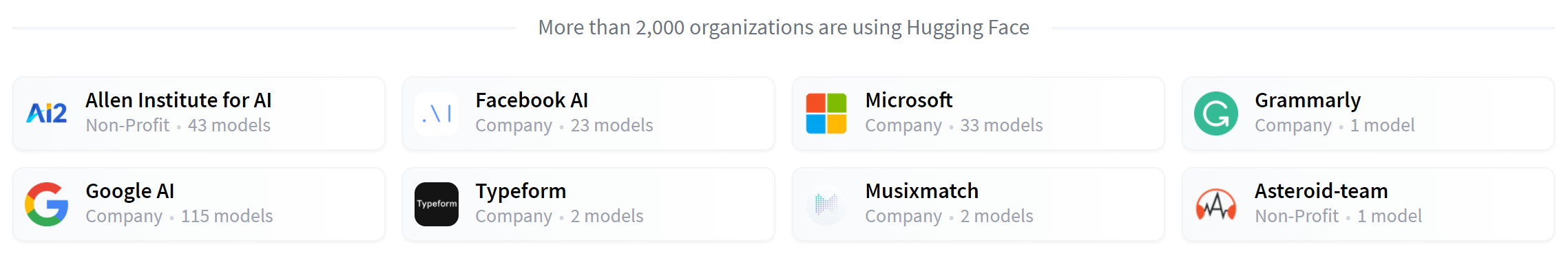
Transformer models are used to solve all kinds of tasks across different modalities, including natural language processing (NLP), computer vision, audio processing, and more. Here are some of the companies and organizations using Hugging Face and Transformer models, who also contribute back to the community by sharing their models:
The 🤗 Transformers library provides the functionality to create and use those shared models. The Model Hub contains millions of pretrained models that anyone can download and use. You can also upload your own models to the Hub!
[!TIP] ⚠️ The Hugging Face Hub is not limited to Transformer models. Anyone can share any kind of models or datasets they want! Create a huggingface.co account to benefit from all available features!
Before diving into how Transformer models work under the hood, let’s look at a few examples of how they can be used to solve some interesting NLP problems.
Working with pipelines
The most basic object in the 🤗 Transformers library is the pipeline() function. It connects a model with its necessary preprocessing and postprocessing steps, allowing us to directly input any text and get an intelligible answer:
from transformers import pipeline

classifier = pipeline("sentiment-analysis")
classifier("I've been waiting for a HuggingFace course my whole life.")
[{'label': 'POSITIVE', 'score': 0.9598047137260437}]
We can even pass several sentences!
classifier(
    ["I've been waiting for a HuggingFace course my whole life.", "I hate this so much!"]
)
[{'label': 'POSITIVE', 'score': 0.9598047137260437},
 {'label': 'NEGATIVE', 'score': 0.9994558095932007}]
By default, this pipeline selects a particular pretrained model that has been fine-tuned for sentiment analysis in English. The model is downloaded and cached when you create the classifier object. If you rerun the command, the cached model will be used instead and there is no need to download the model again.
There are three main steps involved when you pass some text to a pipeline:
- The text is preprocessed into a format the model can understand.
- The preprocessed inputs are passed to the model.
- The predictions of the model are post-processed, so you can make sense of them.
Available pipelines for different modalities
The pipeline() function supports multiple modalities, allowing you to work with text, images, audio, and even multimodal tasks. In this course we’ll focus on text tasks, but it’s useful to understand the transformer architecture’s potential, so we’ll briefly outline it.
Here’s an overview of what’s available:
[!TIP] For a full and updated list of pipelines, see the 🤗 Transformers documentation.
Text pipelines
text-generation: Generate text from a prompttext-classification: Classify text into predefined categoriessummarization: Create a shorter version of a text while preserving key informationtranslation: Translate text from one language to anotherzero-shot-classification: Classify text without prior training on specific labelsfeature-extraction: Extract vector representations of text
Image pipelines
image-to-text: Generate text descriptions of imagesimage-classification: Identify objects in an imageobject-detection: Locate and identify objects in images
Audio pipelines
automatic-speech-recognition: Convert speech to textaudio-classification: Classify audio into categoriestext-to-speech: Convert text to spoken audio
Multimodal pipelines
image-text-to-text: Respond to an image based on a text prompt
Let’s explore some of these pipelines in more detail!
Zero-shot classification
We’ll start by tackling a more challenging task where we need to classify texts that haven’t been labelled. This is a common scenario in real-world projects because annotating text is usually time-consuming and requires domain expertise. For this use case, the zero-shot-classification pipeline is very powerful: it allows you to specify which labels to use for the classification, so you don’t have to rely on the labels of the pretrained model. You’ve already seen how the model can classify a sentence as positive or negative using those two labels — but it can also classify the text using any other set of labels you like.
from transformers import pipeline

classifier = pipeline("zero-shot-classification")
classifier(
    "This is a course about the Transformers library",
    candidate_labels=["education", "politics", "business"],
)
{'sequence': 'This is a course about the Transformers library',
 'labels': ['education', 'business', 'politics'],
 'scores': [0.8445963859558105, 0.111976258456707, 0.043427448719739914]}
This pipeline is called zero-shot because you don’t need to fine-tune the model on your data to use it. It can directly return probability scores for any list of labels you want!
[!TIP] ✏️ Try it out! Play around with your own sequences and labels and see how the model behaves.
Text generation
Now let’s see how to use a pipeline to generate some text. The main idea here is that you provide a prompt and the model will auto-complete it by generating the remaining text. This is similar to the predictive text feature that is found on many phones. Text generation involves randomness, so it’s normal if you don’t get the same results as shown below.
from transformers import pipeline

generator = pipeline("text-generation")
generator("In this course, we will teach you how to")
[{'generated_text': 'In this course, we will teach you how to understand and use '
                    'data flow and data interchange when handling user data. We '
                    'will be working with one or more of the most commonly used '
                    'data flows — data flows of various types, as seen by the '
                    'HTTP'}]
You can control how many different sequences are generated with the argument num_return_sequences and the total length of the output text with the argument max_length.
[!TIP] ✏️ Try it out! Use the
num_return_sequencesandmax_lengtharguments to generate two sentences of 15 words each.
Using any model from the Hub in a pipeline
The previous examples used the default model for the task at hand, but you can also choose a particular model from the Hub to use in a pipeline for a specific task — say, text generation. Go to the Model Hub and click on the corresponding tag on the left to display only the supported models for that task. You should get to a page like this one.
Let’s try the HuggingFaceTB/SmolLM2-360M model! Here’s how to load it in the same pipeline as before:
from transformers import pipeline

generator = pipeline("text-generation", model="HuggingFaceTB/SmolLM2-360M")
generator(
    "In this course, we will teach you how to",
    max_length=30,
    num_return_sequences=2,
)
[{'generated_text': 'In this course, we will teach you how to manipulate the world and '
                    'move your mental and physical capabilities to your advantage.'},
 {'generated_text': 'In this course, we will teach you how to become an expert and '
                    'practice realtime, and with a hands on experience on both real '
                    'time and real'}]
You can refine your search for a model by clicking on the language tags, and pick a model that will generate text in another language. The Model Hub even contains checkpoints for multilingual models that support several languages.
Once you select a model by clicking on it, you’ll see that there is a widget enabling you to try it directly online. This way you can quickly test the model’s capabilities before downloading it.
[!TIP] ✏️ Try it out! Use the filters to find a text generation model for another language. Feel free to play with the widget and use it in a pipeline!
Inference Providers
All the models can be tested directly through your browser using the Inference Providers, which is available on the Hugging Face website. You can play with the model directly on this page by inputting custom text and watching the model process the input data.
Inference Providers that powers the widget is also available as a paid product, which comes in handy if you need it for your workflows. See the pricing page for more details.
Mask filling
The next pipeline you’ll try is fill-mask. The idea of this task is to fill in the blanks in a given text:
from transformers import pipeline

unmasker = pipeline("fill-mask")
unmasker("This course will teach you all about <mask> models.", top_k=2)
[{'sequence': 'This course will teach you all about mathematical models.',
  'score': 0.19619831442832947,
  'token': 30412,
  'token_str': ' mathematical'},
 {'sequence': 'This course will teach you all about computational models.',
  'score': 0.04052725434303284,
  'token': 38163,
  'token_str': ' computational'}]
The top_k argument controls how many possibilities you want to be displayed. Note that here the model fills in the special <mask> word, which is often referred to as a mask token. Other mask-filling models might have different mask tokens, so it’s always good to verify the proper mask word when exploring other models. One way to check it is by looking at the mask word used in the widget.
[!TIP] ✏️ Try it out! Search for the
bert-base-casedmodel on the Hub and identify its mask word in the Inference API widget. What does this model predict for the sentence in ourpipelineexample above?
Named entity recognition
Named entity recognition (NER) is a task where the model has to find which parts of the input text correspond to entities such as persons, locations, or organizations. Let’s look at an example:
from transformers import pipeline

ner = pipeline("ner", aggregation_strategy="simple")
ner("My name is Sylvain and I work at Hugging Face in Brooklyn.")
[{'entity_group': 'PER', 'score': 0.99816, 'word': 'Sylvain', 'start': 11, 'end': 18},
 {'entity_group': 'ORG', 'score': 0.97960, 'word': 'Hugging Face', 'start': 33, 'end': 45},
 {'entity_group': 'LOC', 'score': 0.99321, 'word': 'Brooklyn', 'start': 49, 'end': 57}
]
Here the model correctly identified that Sylvain is a person (PER), Hugging Face an organization (ORG), and Brooklyn a location (LOC).
We pass the option aggregation_strategy="simple" in the pipeline creation function to tell the pipeline to regroup together the parts of the sentence that correspond to the same entity: here the model correctly grouped “Hugging” and “Face” as a single organization, even though the name consists of multiple words. In fact, as we will see in the next chapter, the preprocessing even splits some words into smaller parts. For instance, Sylvain is split into four pieces: S, ##yl, ##va, and ##in. In the post-processing step, the pipeline successfully regrouped those pieces.
[!TIP] ✏️ Try it out! Search the Model Hub for a model able to do part-of-speech tagging (usually abbreviated as POS) in English. What does this model predict for the sentence in the example above?
Question answering
The question-answering pipeline answers questions using information from a given context:
from transformers import pipeline

question_answerer = pipeline("question-answering")
question_answerer(
    question="Where do I work?",
    context="My name is Sylvain and I work at Hugging Face in Brooklyn",
)
{'score': 0.6385916471481323, 'start': 33, 'end': 45, 'answer': 'Hugging Face'}
Note that this pipeline works by extracting information from the provided context; it does not generate the answer.
Summarization
Summarization is the task of reducing a text into a shorter text while keeping all (or most) of the important aspects referenced in the text. Here’s an example:
from transformers import pipeline

summarizer = pipeline("summarization")
summarizer(
    """
    America has changed dramatically during recent years. Not only has the number of
    graduates in traditional engineering disciplines such as mechanical, civil,
    electrical, chemical, and aeronautical engineering declined, but in most of
    the premier American universities engineering curricula now concentrate on
    and encourage largely the study of engineering science. As a result, there
    are declining offerings in engineering subjects dealing with infrastructure,
    the environment, and related issues, and greater concentration on high
    technology subjects, largely supporting increasingly complex scientific
    developments. While the latter is important, it should not be at the expense
    of more traditional engineering.

    Rapidly developing economies such as China and India, as well as other
    industrial countries in Europe and Asia, continue to encourage and advance
    the teaching of engineering. Both China and India, respectively, graduate
    six and eight times as many traditional engineers as does the United States.
    Other industrial countries at minimum maintain their output, while America
    suffers an increasingly serious decline in the number of engineering graduates
    and a lack of well-educated engineers.
"""
)
[{'summary_text': ' America has changed dramatically during recent years . The '
                  'number of engineering graduates in the U.S. has declined in '
                  'traditional engineering disciplines such as mechanical, civil '
                  ', electrical, chemical, and aeronautical engineering . Rapidly '
                  'developing economies such as China and India, as well as other '
                  'industrial countries in Europe and Asia, continue to encourage '
                  'and advance engineering .'}]
Like with text generation, you can specify a max_length or a min_length for the result.
Translation
For translation, you can use a default model if you provide a language pair in the task name (such as "translation_en_to_fr"), but the easiest way is to pick the model you want to use on the Model Hub. Here we’ll try translating from French to English:
from transformers import pipeline

translator = pipeline("translation", model="Helsinki-NLP/opus-mt-fr-en")
translator("Ce cours est produit par Hugging Face.")
[{'translation_text': 'This course is produced by Hugging Face.'}]
Like with text generation and summarization, you can specify a max_length or a min_length for the result.
[!TIP] ✏️ Try it out! Search for translation models in other languages and try to translate the previous sentence into a few different languages.
Image and audio pipelines
Beyond text, Transformer models can also work with images and audio. Here are a few examples:
Image classification
from transformers import pipeline

image_classifier = pipeline(
    task="image-classification", model="google/vit-base-patch16-224"
)
result = image_classifier(
    "https://huggingface.co/datasets/huggingface/documentation-images/resolve/main/pipeline-cat-chonk.jpeg"
)
print(result)
[{'label': 'lynx, catamount', 'score': 0.43350091576576233},
 {'label': 'cougar, puma, catamount, mountain lion, painter, panther, Felis concolor',
  'score': 0.034796204417943954},
 {'label': 'snow leopard, ounce, Panthera uncia',
  'score': 0.03240183740854263},
 {'label': 'Egyptian cat', 'score': 0.02394474856555462},
 {'label': 'tiger cat', 'score': 0.02288915030658245}]
Automatic speech recognition
from transformers import pipeline

transcriber = pipeline(
    task="automatic-speech-recognition", model="openai/whisper-large-v3"
)
result = transcriber(
    "https://huggingface.co/datasets/Narsil/asr_dummy/resolve/main/mlk.flac"
)
print(result)
{'text': ' I have a dream that one day this nation will rise up and live out the true meaning of its creed.'}
Combining data from multiple sources
One powerful application of Transformer models is their ability to combine and process data from multiple sources. This is especially useful when you need to:
- Search across multiple databases or repositories
- Consolidate information from different formats (text, images, audio)
- Create a unified view of related information
For example, you could build a system that:
- Searches for information across databases in multiple modalities like text and image.
- Combines results from different sources into a single coherent response. For example, from an audio file and text description.
- Presents the most relevant information from a database of documents and metadata.
Conclusion
The pipelines shown in this chapter are mostly for demonstrative purposes. They were programmed for specific tasks and cannot perform variations of them. In the next chapter, you’ll learn what’s inside a pipeline() function and how to customize its behavior.
4. How do Transformers work?
In this section, we will take a look at the architecture of Transformer models and dive deeper into the concepts of attention, encoder-decoder architecture, and more.
[!WARNING] 🚀 We’re taking things up a notch here. This section is detailed and technical, so don’t worry if you don’t understand everything right away. We’ll come back to these concepts later in the course.
A bit of Transformer history
Here are some reference points in the (short) history of Transformer models:


The Transformer architecture was introduced in June 2017. The focus of the original research was on translation tasks. This was followed by the introduction of several influential models, including:
June 2018: GPT, the first pretrained Transformer model, used for fine-tuning on various NLP tasks and obtained state-of-the-art results
October 2018: BERT, another large pretrained model, this one designed to produce better summaries of sentences (more on this in the next chapter!)
February 2019: GPT-2, an improved (and bigger) version of GPT that was not immediately publicly released due to ethical concerns
October 2019: T5, A multi-task focused implementation of the sequence-to-sequence Transformer architecture.
May 2020, GPT-3, an even bigger version of GPT-2 that is able to perform well on a variety of tasks without the need for fine-tuning (called zero-shot learning)
January 2022: InstructGPT, a version of GPT-3 that was trained to follow instructions better.
January 2023: Llama, a large language model that is able to generate text in a variety of languages.
March 2023: Mistral, a 7-billion-parameter language model that outperforms Llama 2 13B across all evaluated benchmarks, leveraging grouped-query attention for faster inference and sliding window attention to handle sequences of arbitrary length.
May 2024: Gemma 2, a family of lightweight, state-of-the-art open models ranging from 2B to 27B parameters that incorporate interleaved local-global attentions and group-query attention, with smaller models trained using knowledge distillation to deliver performance competitive with models 2-3 times larger.
November 2024: SmolLM2, a state-of-the-art small language model (135 million to 1.7 billion parameters) that achieves impressive performance despite its compact size, and unlocking new possibilities for mobile and edge devices.
This list is far from comprehensive, and is just meant to highlight a few of the different kinds of Transformer models. Broadly, they can be grouped into three categories:
- GPT-like (also called auto-regressive Transformer models)
- BERT-like (also called auto-encoding Transformer models)
- T5-like (also called sequence-to-sequence Transformer models)
We will dive into these families in more depth later on.
Transformers are language models
All the Transformer models mentioned above (GPT, BERT, T5, etc.) have been trained as language models. This means they have been trained on large amounts of raw text in a self-supervised fashion.
Self-supervised learning is a type of training in which the objective is automatically computed from the inputs of the model. That means that humans are not needed to label the data!
This type of model develops a statistical understanding of the language it has been trained on, but it’s less useful for specific practical tasks. Because of this, the general pretrained model then goes through a process called transfer learning or fine-tuning. During this process, the model is fine-tuned in a supervised way – that is, using human-annotated labels – on a given task.
An example of a task is predicting the next word in a sentence having read the n previous words. This is called causal language modeling because the output depends on the past and present inputs, but not the future ones.

Another example is masked language modeling, in which the model predicts a masked word in the sentence.


Transformers are big models
Apart from a few outliers (like DistilBERT), the general strategy to achieve better performance is by increasing the models’ sizes as well as the amount of data they are pretrained on.
Unfortunately, training a model, especially a large one, requires a large amount of data. This becomes very costly in terms of time and compute resources. It even translates to environmental impact, as can be seen in the following graph.


And this is showing a project for a (very big) model led by a team consciously trying to reduce the environmental impact of pretraining. The footprint of running lots of trials to get the best hyperparameters would be even higher.
Imagine if each time a research team, a student organization, or a company wanted to train a model, it did so from scratch. This would lead to huge, unnecessary global costs!
This is why sharing language models is paramount: sharing the trained weights and building on top of already trained weights reduces the overall compute cost and carbon footprint of the community.
By the way, you can evaluate the carbon footprint of your models’ training through several tools. For example ML CO2 Impact or Code Carbon which is integrated in 🤗 Transformers. To learn more about this, you can read this blog post which will show you how to generate an emissions.csv file with an estimate of the footprint of your training, as well as the documentation of 🤗 Transformers addressing this topic.
Transfer Learning
Pretraining is the act of training a model from scratch: the weights are randomly initialized, and the training starts without any prior knowledge.

This pretraining is usually done on very large amounts of data. Therefore, it requires a very large corpus of data, and training can take up to several weeks.
Fine-tuning, on the other hand, is the training done after a model has been pretrained. To perform fine-tuning, you first acquire a pretrained language model, then perform additional training with a dataset specific to your task. Wait – why not simply train the model for your final use case from the start (scratch)? There are a couple of reasons:
- The pretrained model was already trained on a dataset that has some similarities with the fine-tuning dataset. The fine-tuning process is thus able to take advantage of knowledge acquired by the initial model during pretraining (for instance, with NLP problems, the pretrained model will have some kind of statistical understanding of the language you are using for your task).
- Since the pretrained model was already trained on lots of data, the fine-tuning requires way less data to get decent results.
- For the same reason, the amount of time and resources needed to get good results are much lower.
For example, one could leverage a pretrained model trained on the English language and then fine-tune it on an arXiv corpus, resulting in a science/research-based model. The fine-tuning will only require a limited amount of data: the knowledge the pretrained model has acquired is “transferred,” hence the term transfer learning.


Fine-tuning a model therefore has lower time, data, financial, and environmental costs. It is also quicker and easier to iterate over different fine-tuning schemes, as the training is less constraining than a full pretraining.
This process will also achieve better results than training from scratch (unless you have lots of data), which is why you should always try to leverage a pretrained model – one as close as possible to the task you have at hand – and fine-tune it.
General Transformer architecture
In this section, we’ll go over the general architecture of the Transformer model. Don’t worry if you don’t understand some of the concepts; there are detailed sections later covering each of the components.
The model is primarily composed of two blocks:
- Encoder (left): The encoder receives an input and builds a representation of it (its features). This means that the model is optimized to acquire understanding from the input.
- Decoder (right): The decoder uses the encoder’s representation (features) along with other inputs to generate a target sequence. This means that the model is optimized for generating outputs.


Each of these parts can be used independently, depending on the task:
- Encoder-only models: Good for tasks that require understanding of the input, such as sentence classification and named entity recognition.
- Decoder-only models: Good for generative tasks such as text generation.
- Encoder-decoder models or sequence-to-sequence models: Good for generative tasks that require an input, such as translation or summarization.
We will dive into those architectures independently in later sections.
Attention layers
A key feature of Transformer models is that they are built with special layers called attention layers. In fact, the title of the paper introducing the Transformer architecture was “Attention Is All You Need”! We will explore the details of attention layers later in the course; for now, all you need to know is that this layer will tell the model to pay specific attention to certain words in the sentence you passed it (and more or less ignore the others) when dealing with the representation of each word.
To put this into context, consider the task of translating text from English to French. Given the input “You like this course”, a translation model will need to also attend to the adjacent word “You” to get the proper translation for the word “like”, because in French the verb “like” is conjugated differently depending on the subject. The rest of the sentence, however, is not useful for the translation of that word. In the same vein, when translating “this” the model will also need to pay attention to the word “course”, because “this” translates differently depending on whether the associated noun is masculine or feminine. Again, the other words in the sentence will not matter for the translation of “course”. With more complex sentences (and more complex grammar rules), the model would need to pay special attention to words that might appear farther away in the sentence to properly translate each word.
The same concept applies to any task associated with natural language: a word by itself has a meaning, but that meaning is deeply affected by the context, which can be any other word (or words) before or after the word being studied.
Now that you have an idea of what attention layers are all about, let’s take a closer look at the Transformer architecture.
The original architecture
The Transformer architecture was originally designed for translation. During training, the encoder receives inputs (sentences) in a certain language, while the decoder receives the same sentences in the desired target language. In the encoder, the attention layers can use all the words in a sentence (since, as we just saw, the translation of a given word can be dependent on what is after as well as before it in the sentence). The decoder, however, works sequentially and can only pay attention to the words in the sentence that it has already translated (so, only the words before the word currently being generated). For example, when we have predicted the first three words of the translated target, we give them to the decoder which then uses all the inputs of the encoder to try to predict the fourth word.
To speed things up during training (when the model has access to target sentences), the decoder is fed the whole target, but it is not allowed to use future words (if it had access to the word at position 2 when trying to predict the word at position 2, the problem would not be very hard!). For instance, when trying to predict the fourth word, the attention layer will only have access to the words in positions 1 to 3.
The original Transformer architecture looked like this, with the encoder on the left and the decoder on the right:


Note that the first attention layer in a decoder block pays attention to all (past) inputs to the decoder, but the second attention layer uses the output of the encoder. It can thus access the whole input sentence to best predict the current word. This is very useful as different languages can have grammatical rules that put the words in different orders, or some context provided later in the sentence may be helpful to determine the best translation of a given word.
The attention mask can also be used in the encoder/decoder to prevent the model from paying attention to some special words – for instance, the special padding word used to make all the inputs the same length when batching together sentences.
Architectures vs. checkpoints
As we dive into Transformer models in this course, you’ll see mentions of architectures and checkpoints as well as models. These terms all have slightly different meanings:
- Architecture: This is the skeleton of the model – the definition of each layer and each operation that happens within the model.
- Checkpoints: These are the weights that will be loaded in a given architecture.
- Model: This is an umbrella term that isn’t as precise as “architecture” or “checkpoint”: it can mean both. This course will specify architecture or checkpoint when it matters to reduce ambiguity.
For example, BERT is an architecture while bert-base-cased, a set of weights trained by the Google team for the first release of BERT, is a checkpoint. However, one can say “the BERT model” and “the bert-base-cased model.”
5. How 🤗 Transformers solve tasks
In Transformers, what can they do?, you learned about natural language processing (NLP), speech and audio, computer vision tasks, and some important applications of them. This page will look closely at how models solve these tasks and explain what’s happening under the hood. There are many ways to solve a given task, some models may implement certain techniques or even approach the task from a new angle, but for Transformer models, the general idea is the same. Owing to its flexible architecture, most models are a variant of an encoder, a decoder, or an encoder-decoder structure.
[!TIP] Before diving into specific architectural variants, it’s helpful to understand that most tasks follow a similar pattern: input data is processed through a model, and the output is interpreted for a specific task. The differences lie in how the data is prepared, what model architecture variant is used, and how the output is processed.
To explain how tasks are solved, we’ll walk through what goes on inside the model to output useful predictions. We’ll cover the following models and their corresponding tasks:
- Wav2Vec2 for audio classification and automatic speech recognition (ASR)
- Vision Transformer (ViT) and ConvNeXT for image classification
- DETR for object detection
- Mask2Former for image segmentation
- GLPN for depth estimation
- BERT for NLP tasks like text classification, token classification and question answering that use an encoder
- GPT2 for NLP tasks like text generation that use a decoder
- BART for NLP tasks like summarization and translation that use an encoder-decoder
[!TIP] Before you go further, it is good to have some basic knowledge of the original Transformer architecture. Knowing how encoders, decoders, and attention work will aid you in understanding how different Transformer models work. Be sure to check out our the previous section for more information!
Transformer models for language
Language models are at the heart of modern NLP. They’re designed to understand and generate human language by learning the statistical patterns and relationships between words or tokens in text.
The Transformer was initially designed for machine translation, and since then, it has become the default architecture for solving all AI tasks. Some tasks lend themselves to the Transformer’s encoder structure, while others are better suited for the decoder. Still, other tasks make use of both the Transformer’s encoder-decoder structure.
How language models work
Language models work by being trained to predict the probability of a word given the context of surrounding words. This gives them a foundational understanding of language that can generalize to other tasks.
There are two main approaches for training a transformer model:
Masked language modeling (MLM): Used by encoder models like BERT, this approach randomly masks some tokens in the input and trains the model to predict the original tokens based on the surrounding context. This allows the model to learn bidirectional context (looking at words both before and after the masked word).
Causal language modeling (CLM): Used by decoder models like GPT, this approach predicts the next token based on all previous tokens in the sequence. The model can only use context from the left (previous tokens) to predict the next token.
Types of language models
In the Transformers library, language models generally fall into three architectural categories:
Encoder-only models (like BERT): These models use a bidirectional approach to understand context from both directions. They’re best suited for tasks that require deep understanding of text, such as classification, named entity recognition, and question answering.
Decoder-only models (like GPT, Llama): These models process text from left to right and are particularly good at text generation tasks. They can complete sentences, write essays, or even generate code based on a prompt.
Encoder-decoder models (like T5, BART): These models combine both approaches, using an encoder to understand the input and a decoder to generate output. They excel at sequence-to-sequence tasks like translation, summarization, and question answering.

As we covered in the previous section, language models are typically pretrained on large amounts of text data in a self-supervised manner (without human annotations), then fine-tuned on specific tasks. This approach, known as transfer learning, allows these models to adapt to many different NLP tasks with relatively small amounts of task-specific data.
In the following sections, we’ll explore specific model architectures and how they’re applied to various tasks across speech, vision, and text domains.
[!TIP] Understanding which part of the Transformer architecture (encoder, decoder, or both) is best suited for a particular NLP task is key to choosing the right model. Generally, tasks requiring bidirectional context use encoders, tasks generating text use decoders, and tasks converting one sequence to another use encoder-decoders.
Text generation
Text generation involves creating coherent and contextually relevant text based on a prompt or input.
GPT-2 is a decoder-only model pretrained on a large amount of text. It can generate convincing (though not always true!) text given a prompt and complete other NLP tasks like question answering despite not being explicitly trained to.
GPT-2 uses byte pair encoding (BPE) to tokenize words and generate a token embedding. Positional encodings are added to the token embeddings to indicate the position of each token in the sequence. The input embeddings are passed through multiple decoder blocks to output some final hidden state. Within each decoder block, GPT-2 uses a masked self-attention layer which means GPT-2 can’t attend to future tokens. It is only allowed to attend to tokens on the left. This is different from BERT’s [
mask] token because, in masked self-attention, an attention mask is used to set the score to0for future tokens.The output from the decoder is passed to a language modeling head, which performs a linear transformation to convert the hidden states into logits. The label is the next token in the sequence, which are created by shifting the logits to the right by one. The cross-entropy loss is calculated between the shifted logits and the labels to output the next most likely token.
GPT-2’s pretraining objective is based entirely on causal language modeling, predicting the next word in a sequence. This makes GPT-2 especially good at tasks that involve generating text.
Ready to try your hand at text generation? Check out our complete causal language modeling guide to learn how to finetune DistilGPT-2 and use it for inference!
[!TIP] For more information about text generation, check out the text generation strategies guide!
Text classification
Text classification involves assigning predefined categories to text documents, such as sentiment analysis, topic classification, or spam detection.
BERT is an encoder-only model and is the first model to effectively implement deep bidirectionality to learn richer representations of the text by attending to words on both sides.
BERT uses WordPiece tokenization to generate a token embedding of the text. To tell the difference between a single sentence and a pair of sentences, a special
[SEP]token is added to differentiate them. A special[CLS]token is added to the beginning of every sequence of text. The final output with the[CLS]token is used as the input to the classification head for classification tasks. BERT also adds a segment embedding to denote whether a token belongs to the first or second sentence in a pair of sentences.BERT is pretrained with two objectives: masked language modeling and next-sentence prediction. In masked language modeling, some percentage of the input tokens are randomly masked, and the model needs to predict these. This solves the issue of bidirectionality, where the model could cheat and see all the words and “predict” the next word. The final hidden states of the predicted mask tokens are passed to a feedforward network with a softmax over the vocabulary to predict the masked word.
The second pretraining object is next-sentence prediction. The model must predict whether sentence B follows sentence A. Half of the time sentence B is the next sentence, and the other half of the time, sentence B is a random sentence. The prediction, whether it is the next sentence or not, is passed to a feedforward network with a softmax over the two classes (
IsNextandNotNext).The input embeddings are passed through multiple encoder layers to output some final hidden states.
To use the pretrained model for text classification, add a sequence classification head on top of the base BERT model. The sequence classification head is a linear layer that accepts the final hidden states and performs a linear transformation to convert them into logits. The cross-entropy loss is calculated between the logits and target to find the most likely label.
Ready to try your hand at text classification? Check out our complete text classification guide to learn how to finetune DistilBERT and use it for inference!
Token classification
Token classification involves assigning a label to each token in a sequence, such as in named entity recognition or part-of-speech tagging.
To use BERT for token classification tasks like named entity recognition (NER), add a token classification head on top of the base BERT model. The token classification head is a linear layer that accepts the final hidden states and performs a linear transformation to convert them into logits. The cross-entropy loss is calculated between the logits and each token to find the most likely label.
Ready to try your hand at token classification? Check out our complete token classification guide to learn how to finetune DistilBERT and use it for inference!
Question answering
Question answering involves finding the answer to a question within a given context or passage.
To use BERT for question answering, add a span classification head on top of the base BERT model. This linear layer accepts the final hidden states and performs a linear transformation to compute the span start and end logits corresponding to the answer. The cross-entropy loss is calculated between the logits and the label position to find the most likely span of text corresponding to the answer.
Ready to try your hand at question answering? Check out our complete question answering guide to learn how to finetune DistilBERT and use it for inference!
[!TIP] 💡 Notice how easy it is to use BERT for different tasks once it’s been pretrained. You only need to add a specific head to the pretrained model to manipulate the hidden states into your desired output!
Summarization
Summarization involves condensing a longer text into a shorter version while preserving its key information and meaning.
Encoder-decoder models like BART and T5 are designed for the sequence-to-sequence pattern of a summarization task. We’ll explain how BART works in this section, and then you can try finetuning T5 at the end.
BART’s encoder architecture is very similar to BERT and accepts a token and positional embedding of the text. BART is pretrained by corrupting the input and then reconstructing it with the decoder. Unlike other encoders with specific corruption strategies, BART can apply any type of corruption. The text infilling corruption strategy works the best though. In text infilling, a number of text spans are replaced with a single [
mask] token. This is important because the model has to predict the masked tokens, and it teaches the model to predict the number of missing tokens. The input embeddings and masked spans are passed through the encoder to output some final hidden states, but unlike BERT, BART doesn’t add a final feedforward network at the end to predict a word.The encoder’s output is passed to the decoder, which must predict the masked tokens and any uncorrupted tokens from the encoder’s output. This gives additional context to help the decoder restore the original text. The output from the decoder is passed to a language modeling head, which performs a linear transformation to convert the hidden states into logits. The cross-entropy loss is calculated between the logits and the label, which is just the token shifted to the right.
Ready to try your hand at summarization? Check out our complete summarization guide to learn how to finetune T5 and use it for inference!
[!TIP] For more information about text generation, check out the text generation strategies guide!
Translation
Translation involves converting text from one language to another while preserving its meaning. Translation is another example of a sequence-to-sequence task, which means you can use an encoder-decoder model like BART or T5 to do it. We’ll explain how BART works in this section, and then you can try finetuning T5 at the end.
BART adapts to translation by adding a separate randomly initialized encoder to map a source language to an input that can be decoded into the target language. This new encoder’s embeddings are passed to the pretrained encoder instead of the original word embeddings. The source encoder is trained by updating the source encoder, positional embeddings, and input embeddings with the cross-entropy loss from the model output. The model parameters are frozen in this first step, and all the model parameters are trained together in the second step. BART has since been followed up by a multilingual version, mBART, intended for translation and pretrained on many different languages.
Ready to try your hand at translation? Check out our complete translation guide to learn how to finetune T5 and use it for inference!
[!TIP] As you’ve seen throughout this guide, many models follow similar patterns despite addressing different tasks. Understanding these common patterns can help you quickly grasp how new models work and how to adapt existing models to your specific needs.
Modalities beyond text
Transformers are not limited to text. They can also be applied to other modalities like speech and audio, images, and video. Of course, on this course we will focus on text, but we can briefly introduce the other modalities.
Speech and audio
Let’s start by exploring how Transformer models handle speech and audio data, which presents unique challenges compared to text or images.
Whisper is a encoder-decoder (sequence-to-sequence) transformer pretrained on 680,000 hours of labeled audio data. This amount of pretraining data enables zero-shot performance on audio tasks in English and many other languages. The decoder allows Whisper to map the encoders learned speech representations to useful outputs, such as text, without additional fine-tuning. Whisper just works out of the box.

Diagram is from Whisper paper.
This model has two main components:
An encoder processes the input audio. The raw audio is first converted into a log-Mel spectrogram. This spectrogram is then passed through a Transformer encoder network.
A decoder takes the encoded audio representation and autoregressively predicts the corresponding text tokens. It’s a standard Transformer decoder trained to predict the next text token given the previous tokens and the encoder output. Special tokens are used at the beginning of the decoder input to steer the model towards specific tasks like transcription, translation, or language identification.
Whisper was pretrained on a massive and diverse dataset of 680,000 hours of labeled audio data collected from the web. This large-scale, weakly supervised pretraining is the key to its strong zero-shot performance across many languages and tasks.
Now that Whisper is pretrained, you can use it directly for zero-shot inference or finetune it on your data for improved performance on specific tasks like automatic speech recognition or speech translation!
[!TIP] The key innovation in Whisper is its training on an unprecedented scale of diverse, weakly supervised audio data from the internet. This allows it to generalize remarkably well to different languages, accents, and tasks without task-specific finetuning.
Automatic speech recognition
To use the pretrained model for automatic speech recognition, you leverage its full encoder-decoder structure. The encoder processes the audio input, and the decoder autoregressively generates the transcript token by token. When fine-tuning, the model is typically trained using a standard sequence-to-sequence loss (like cross-entropy) to predict the correct text tokens based on the audio input.
The easiest way to use a fine-tuned model for inference is within a pipeline.
from transformers import pipeline

transcriber = pipeline(
    task="automatic-speech-recognition", model="openai/whisper-base.en"
)
transcriber("https://huggingface.co/datasets/Narsil/asr_dummy/resolve/main/mlk.flac")
# Output: {'text': ' I have a dream that one day this nation will rise up and live out the true meaning of its creed.'}
Ready to try your hand at automatic speech recognition? Check out our complete automatic speech recognition guide to learn how to finetune Whisper and use it for inference!
Computer vision
Now let’s move on to computer vision tasks, which deal with understanding and interpreting visual information from images or videos.
There are two ways to approach computer vision tasks:
- Split an image into a sequence of patches and process them in parallel with a Transformer.
- Use a modern CNN, like ConvNeXT, which relies on convolutional layers but adopts modern network designs.
[!TIP] A third approach mixes Transformers with convolutions (for example, Convolutional Vision Transformer or LeViT). We won’t discuss those because they just combine the two approaches we examine here.
ViT and ConvNeXT are commonly used for image classification, but for other vision tasks like object detection, segmentation, and depth estimation, we’ll look at DETR, Mask2Former and GLPN, respectively; these models are better suited for those tasks.
Image classification
Image classification is one of the fundamental computer vision tasks. Let’s see how different model architectures approach this problem.
ViT and ConvNeXT can both be used for image classification; the main difference is that ViT uses an attention mechanism while ConvNeXT uses convolutions.
ViT replaces convolutions entirely with a pure Transformer architecture. If you’re familiar with the original Transformer, then you’re already most of the way toward understanding ViT.
The main change ViT introduced was in how images are fed to a Transformer:
An image is split into square non-overlapping patches, each of which gets turned into a vector or patch embedding. The patch embeddings are generated from a convolutional 2D layer which creates the proper input dimensions (which for a base Transformer is 768 values for each patch embedding). If you had a 224x224 pixel image, you could split it into 196 16x16 image patches. Just like how text is tokenized into words, an image is “tokenized” into a sequence of patches.
A learnable embedding - a special
[CLS]token - is added to the beginning of the patch embeddings just like BERT. The final hidden state of the[CLS]token is used as the input to the attached classification head; other outputs are ignored. This token helps the model learn how to encode a representation of the image.The last thing to add to the patch and learnable embeddings are the position embeddings because the model doesn’t know how the image patches are ordered. The position embeddings are also learnable and have the same size as the patch embeddings. Finally, all of the embeddings are passed to the Transformer encoder.
The output, specifically only the output with the
[CLS]token, is passed to a multilayer perceptron head (MLP). ViT’s pretraining objective is simply classification. Like other classification heads, the MLP head converts the output into logits over the class labels and calculates the cross-entropy loss to find the most likely class.
Ready to try your hand at image classification? Check out our complete image classification guide to learn how to fine-tune ViT and use it for inference!
[!TIP] Notice the parallel between ViT and BERT: both use a special token (
[CLS]) to capture the overall representation, both add position information to their embeddings, and both use a Transformer encoder to process the sequence of tokens/patches.
6. Transformer Architectures
In the previous sections, we introduced the general Transformer architecture and explored how these models can solve various tasks. Now, let’s take a closer look at the three main architectural variants of Transformer models and understand when to use each one. Then, we look at how those architectures are applied to different language tasks.
In this section, we’re going to dive deeper into the three main architectural variants of Transformer models and understand when to use each one.
[!TIP] Remember that most Transformer models use one of three architectures: encoder-only, decoder-only, or encoder-decoder (sequence-to-sequence). Understanding these differences will help you choose the right model for your specific task.
Encoder models
Encoder models use only the encoder of a Transformer model. At each stage, the attention layers can access all the words in the initial sentence. These models are often characterized as having “bi-directional” attention, and are often called auto-encoding models.
The pretraining of these models usually revolves around somehow corrupting a given sentence (for instance, by masking random words in it) and tasking the model with finding or reconstructing the initial sentence.
Encoder models are best suited for tasks requiring an understanding of the full sentence, such as sentence classification, named entity recognition (and more generally word classification), and extractive question answering.
[!TIP] As we saw in How 🤗 Transformers solve tasks, encoder models like BERT excel at understanding text because they can look at the entire context in both directions. This makes them perfect for tasks where comprehension of the whole input is important.
Representatives of this family of models include:
Decoder models
Decoder models use only the decoder of a Transformer model. At each stage, for a given word the attention layers can only access the words positioned before it in the sentence. These models are often called auto-regressive models.
The pretraining of decoder models usually revolves around predicting the next word in the sentence.
These models are best suited for tasks involving text generation.
[!TIP] Decoder models like GPT are designed to generate text by predicting one token at a time. As we explored in How 🤗 Transformers solve tasks, they can only see previous tokens, which makes them excellent for creative text generation but less ideal for tasks requiring bidirectional understanding.
Representatives of this family of models include:
Modern Large Language Models (LLMs)
Most modern Large Language Models (LLMs) use the decoder-only architecture. These models have grown dramatically in size and capabilities over the past few years, with some of the largest models containing hundreds of billions of parameters.
Modern LLMs are typically trained in two phases:
- Pretraining: The model learns to predict the next token on vast amounts of text data
- Instruction tuning: The model is fine-tuned to follow instructions and generate helpful responses
This approach has led to models that can understand and generate human-like text across a wide range of topics and tasks.
Key capabilities of modern LLMs
Modern decoder-based LLMs have demonstrated impressive capabilities:
| Capability | Description | Example |
|---|---|---|
| Text generation | Creating coherent and contextually relevant text | Writing essays, stories, or emails |
| Summarization | Condensing long documents into shorter versions | Creating executive summaries of reports |
| Translation | Converting text between languages | Translating English to Spanish |
| Question answering | Providing answers to factual questions | “What is the capital of France?” |
| Code generation | Writing or completing code snippets | Creating a function based on a description |
| Reasoning | Working through problems step by step | Solving math problems or logical puzzles |
| Few-shot learning | Learning from a few examples in the prompt | Classifying text after seeing just 2-3 examples |
You can experiment with decoder-based LLMs directly in your browser via model repo pages on the Hub. Here’s an example with the classic GPT-2 (OpenAI’s finest open source model!):
View GPT-2 model on Hugging Face
Sequence-to-sequence models
Encoder-decoder models (also called sequence-to-sequence models) use both parts of the Transformer architecture. At each stage, the attention layers of the encoder can access all the words in the initial sentence, whereas the attention layers of the decoder can only access the words positioned before a given word in the input.
The pretraining of these models can take different forms, but it often involves reconstructing a sentence for which the input has been somehow corrupted (for instance by masking random words). The pretraining of the T5 model consists of replacing random spans of text (that can contain several words) with a single mask special token, and the task is then to predict the text that this mask token replaces.
Sequence-to-sequence models are best suited for tasks revolving around generating new sentences depending on a given input, such as summarization, translation, or generative question answering.
[!TIP] As we saw in How 🤗 Transformers solve tasks, encoder-decoder models like BART and T5 combine the strengths of both architectures. The encoder provides deep bidirectional understanding of the input, while the decoder generates appropriate output text. This makes them perfect for tasks that transform one sequence into another, like translation or summarization.
Practical applications
Sequence-to-sequence models excel at tasks that require transforming one form of text into another while preserving meaning. Some practical applications include:
| Application | Description | Example Model |
|---|---|---|
| Machine translation | Converting text between languages | Marian, T5 |
| Text summarization | Creating concise summaries of longer texts | BART, T5 |
| Data-to-text generation | Converting structured data into natural language | T5 |
| Grammar correction | Fixing grammatical errors in text | T5 |
| Question answering | Generating answers based on context | BART, T5 |
Here’s an interactive demo of a sequence-to-sequence model for translation:
Representatives of this family of models include:
Choosing the right architecture
When working on a specific NLP task, how do you decide which architecture to use? Here’s a quick guide:
| Task | Suggested Architecture | Examples |
|---|---|---|
| Text classification (sentiment, topic) | Encoder | BERT, RoBERTa |
| Text generation (creative writing) | Decoder | GPT, LLaMA |
| Translation | Encoder-Decoder | T5, BART |
| Summarization | Encoder-Decoder | BART, T5 |
| Named entity recognition | Encoder | BERT, RoBERTa |
| Question answering (extractive) | Encoder | BERT, RoBERTa |
| Question answering (generative) | Encoder-Decoder or Decoder | T5, GPT |
| Conversational AI | Decoder | GPT, LLaMA |
[!TIP] When in doubt about which model to use, consider:
- What kind of understanding does your task need? (Bidirectional or unidirectional)
- Are you generating new text or analyzing existing text?
- Do you need to transform one sequence into another?
The answers to these questions will guide you toward the right architecture.
The evolution of LLMs
Large Language Models have evolved rapidly in recent years, with each generation bringing significant improvements in capabilities.
Attention mechanisms
Most transformer models use full attention in the sense that the attention matrix is square. It can be a big computational bottleneck when you have long texts. Longformer and reformer are models that try to be more efficient and use a sparse version of the attention matrix to speed up training.
[!TIP] Standard attention mechanisms have a computational complexity of O(n²), where n is the sequence length. This becomes problematic for very long sequences. The specialized attention mechanisms below help address this limitation.
LSH attention
Reformer uses LSH attention. In the softmax(QK^t), only the biggest elements (in the softmax dimension) of the matrix QK^t are going to give useful contributions. So for each query q in Q, we can consider only the keys k in K that are close to q. A hash function is used to determine if q and k are close. The attention mask is modified to mask the current token (except at the first position), because it will give a query and a key equal (so very similar to each other). Since the hash can be a bit random, several hash functions are used in practice (determined by a n_rounds parameter) and then are averaged together.
Local attention
Longformer uses local attention: often, the local context (e.g., what are the two tokens to the left and right?) is enough to take action for a given token. Also, by stacking attention layers that have a small window, the last layer will have a receptive field of more than just the tokens in the window, allowing them to build a representation of the whole sentence.
Some preselected input tokens are also given global attention: for those few tokens, the attention matrix can access all tokens and this process is symmetric: all other tokens have access to those specific tokens (on top of the ones in their local window). This is shown in Figure 2d of the paper, see below for a sample attention mask:

Using those attention matrices with less parameters then allows the model to have inputs having a bigger sequence length.
Axial positional encodings
Reformer uses axial positional encodings: in traditional transformer models, the positional encoding E is a matrix of size \(l\) by \(d\), \(l\) being the sequence length and \(d\) the dimension of the hidden state. If you have very long texts, this matrix can be huge and take way too much space on the GPU. To alleviate that, axial positional encodings consist of factorizing that big matrix E in two smaller matrices E1 and E2, with dimensions \(l_{1} \times d_{1}\) and \(l_{2} \times d_{2}\), such that \(l_{1} \times l_{2} = l\) and \(d_{1} + d_{2} = d\) (with the product for the lengths, this ends up being way smaller). The embedding for time step \(j\) in E is obtained by concatenating the embeddings for timestep \(j \% l1\) in E1 and \(j // l1\) in E2.
Conclusion
In this section, we’ve explored the three main Transformer architectures and some specialized attention mechanisms. Understanding these architectural differences is crucial for selecting the right model for your specific NLP task.
As we move forward in the course, you’ll get hands-on experience with these different architectures and learn how to fine-tune them for your specific needs. In the next section, we’ll look at some of the limitations and biases present in these models that you should be aware of when deploying them.
8. Deep dive into Text Generation Inference with LLMs
So far, we’ve explored the transformer architecture in relation to a range of discrete tasks, like text classification or summarization. However, Large Language Models are most used for text generation, and this is what we’ll explore in this chapter.
In this page, we’ll explore the core concepts behind LLM inference, providing a comprehensive understanding of how these models generate text and the key components involved in the inference process.
Understanding the Basics
Let’s start with the fundamentals. Inference is the process of using a trained LLM to generate human-like text from a given input prompt. Language models use their knowledge from training to formulate responses one word at a time. The model leverages learned probabilities from billions of parameters to predict and generate the next token in a sequence. This sequential generation is what allows LLMs to produce coherent and contextually relevant text.
The Role of Attention
The attention mechanism is what gives LLMs their ability to understand context and generate coherent responses. When predicting the next word, not every word in a sentence carries equal weight - for example, in the sentence “The capital of France is …“, the words “France” and “capital” are crucial for determining that “Paris” should come next. This ability to focus on relevant information is what we call attention.

This process of identifying the most relevant words to predict the next token has proven to be incredibly effective. Although the basic principle of training LLMs—predicting the next token—has remained generally consistent since BERT and GPT-2, there have been significant advancements in scaling neural networks and making the attention mechanism work for longer and longer sequences, at lower and lower costs.
[!TIP] In short, the attention mechanism is the key to LLMs being able to generate text that is both coherent and context-aware. It sets modern LLMs apart from previous generations of language models.
Context Length and Attention Span
Now that we understand attention, let’s explore how much context an LLM can actually handle. This brings us to context length, or the model’s ‘attention span’.
The context length refers to the maximum number of tokens (words or parts of words) that the LLM can process at once. Think of it as the size of the model’s working memory.
These capabilities are limited by several practical factors:
- The model’s architecture and size
- Available computational resources
- The complexity of the input and desired output
In an ideal world, we could feed unlimited context to the model, but hardware constraints and computational costs make this impractical. This is why different models are designed with different context lengths to balance capability with efficiency.
[!TIP] The context length is the maximum number of tokens the model can consider at once when generating a response.
The Art of Prompting
When we pass information to LLMs, we structure our input in a way that guides the generation of the LLM toward the desired output. This is called prompting.
Understanding how LLMs process information helps us craft better prompts. Since the model’s primary task is to predict the next token by analyzing the importance of each input token, the wording of your input sequence becomes crucial.
[!TIP] Careful design of the prompt makes it easier to guide the generation of the LLM toward the desired output.
The Two-Phase Inference Process
Now that we understand the basic components, let’s dive into how LLMs actually generate text. The process can be broken down into two main phases: prefill and decode. These phases work together like an assembly line, each playing a crucial role in producing coherent text.
The Prefill Phase
The prefill phase is like the preparation stage in cooking - it’s where all the initial ingredients are processed and made ready. This phase involves three key steps:
- Tokenization: Converting the input text into tokens (think of these as the basic building blocks the model understands)
- Embedding Conversion: Transforming these tokens into numerical representations that capture their meaning
- Initial Processing: Running these embeddings through the model’s neural networks to create a rich understanding of the context
This phase is computationally intensive because it needs to process all input tokens at once. Think of it as reading and understanding an entire paragraph before starting to write a response.
You can experiment with different tokenizers in the interactive playground below:
The Decode Phase
After the prefill phase has processed the input, we move to the decode phase - this is where the actual text generation happens. The model generates one token at a time in what we call an autoregressive process (where each new token depends on all previous tokens).
The decode phase involves several key steps that happen for each new token:
- Attention Computation: Looking back at all previous tokens to understand context
- Probability Calculation: Determining the likelihood of each possible next token
- Token Selection: Choosing the next token based on these probabilities
- Continuation Check: Deciding whether to continue or stop generation
This phase is memory-intensive because the model needs to keep track of all previously generated tokens and their relationships.
Sampling Strategies
Now that we understand how the model generates text, let’s explore the various ways we can control this generation process. Just like a writer might choose between being more creative or more precise, we can adjust how the model makes its token selections.
| You can interact with the basic decoding process yourself with SmolLM2 in this Space (remember, it decodes until reaching an EOS token which is **< | im_end | >** for this model): |
Understanding Token Selection: From Probabilities to Token Choices
When the model needs to choose the next token, it starts with raw probabilities (called logits) for every word in its vocabulary. But how do we turn these probabilities into actual choices? Let’s break down the process:

- Raw Logits: Think of these as the model’s initial gut feelings about each possible next word
- Temperature Control: Like a creativity dial - higher settings (>1.0) make choices more random and creative, lower settings (<1.0) make them more focused and deterministic
- Top-p (Nucleus) Sampling: Instead of considering all possible words, we only look at the most likely ones that add up to our chosen probability threshold (e.g., top 90%)
- Top-k Filtering: An alternative approach where we only consider the k most likely next words
Managing Repetition: Keeping Output Fresh
One common challenge with LLMs is their tendency to repeat themselves - much like a speaker who keeps returning to the same points. To address this, we use two types of penalties:
- Presence Penalty: A fixed penalty applied to any token that has appeared before, regardless of how often. This helps prevent the model from reusing the same words.
- Frequency Penalty: A scaling penalty that increases based on how often a token has been used. The more a word appears, the less likely it is to be chosen again.

These penalties are applied early in the token selection process, adjusting the raw probabilities before other sampling strategies are applied. Think of them as gentle nudges encouraging the model to explore new vocabulary.
Controlling Generation Length: Setting Boundaries
Just as a good story needs proper pacing and length, we need ways to control how much text our LLM generates. This is crucial for practical applications - whether we’re generating a tweet-length response or a full blog post.
We can control generation length in several ways:
- Token Limits: Setting minimum and maximum token counts
- Stop Sequences: Defining specific patterns that signal the end of generation
- End-of-Sequence Detection: Letting the model naturally conclude its response
For example, if we want to generate a single paragraph, we might set a maximum of 100 tokens and use “\n\n” as a stop sequence. This ensures our output stays focused and appropriately sized for its purpose.

Beam Search: Looking Ahead for Better Coherence
While the strategies we’ve discussed so far make decisions one token at a time, beam search takes a more holistic approach. Instead of committing to a single choice at each step, it explores multiple possible paths simultaneously - like a chess player thinking several moves ahead.

Here’s how it works:
- At each step, maintain multiple candidate sequences (typically 5-10)
- For each candidate, compute probabilities for the next token
- Keep only the most promising combinations of sequences and next tokens
- Continue this process until reaching the desired length or stop condition
- Select the sequence with the highest overall probability
You can explore beam search visually here:
This approach often produces more coherent and grammatically correct text, though it requires more computational resources than simpler methods.
Practical Challenges and Optimization
As we wrap up our exploration of LLM inference, let’s look at the practical challenges you’ll face when deploying these models, and how to measure and optimize their performance.
Key Performance Metrics
When working with LLMs, four critical metrics will shape your implementation decisions:
- Time to First Token (TTFT): How quickly can you get the first response? This is crucial for user experience and is primarily affected by the prefill phase.
- Time Per Output Token (TPOT): How fast can you generate subsequent tokens? This determines the overall generation speed.
- Throughput: How many requests can you handle simultaneously? This affects scaling and cost efficiency.
- VRAM Usage: How much GPU memory do you need? This often becomes the primary constraint in real-world applications.
The Context Length Challenge
One of the most significant challenges in LLM inference is managing context length effectively. Longer contexts provide more information but come with substantial costs:
- Memory Usage: Grows quadratically with context length
- Processing Speed: Decreases linearly with longer contexts
- Resource Allocation: Requires careful balancing of VRAM usage
Recent models like Qwen2.5-1M offer impressive 1M token context windows, but this comes at the cost of significantly slower inference times. The key is finding the right balance for your specific use case.
(e.g., 4K tokens)
∝ Length²
∝ Length
The KV Cache Optimization
To address these challenges, one of the most powerful optimizations is KV (Key-Value) caching. This technique significantly improves inference speed by storing and reusing intermediate calculations. This optimization:
- Reduces repeated calculations
- Improves generation speed
- Makes long-context generation practical
The trade-off is additional memory usage, but the performance benefits usually far outweigh this cost.
Conclusion
Understanding LLM inference is crucial for effectively deploying and optimizing these powerful models. We’ve covered the key components:
- The fundamental role of attention and context
- The two-phase inference process
- Various sampling strategies for controlling generation
- Practical challenges and optimizations
By mastering these concepts, you’ll be better equipped to build applications that leverage LLMs effectively and efficiently.
Remember that the field of LLM inference is rapidly evolving, with new techniques and optimizations emerging regularly. Stay curious and keep experimenting with different approaches to find what works best for your specific use cases.
9. Bias and limitations
If your intent is to use a pretrained model or a fine-tuned version in production, please be aware that, while these models are powerful tools, they come with limitations. The biggest of these is that, to enable pretraining on large amounts of data, researchers often scrape all the content they can find, taking the best as well as the worst of what is available on the internet.
To give a quick illustration, let’s go back to the example of a fill-mask pipeline with the BERT model:
from transformers import pipeline

unmasker = pipeline("fill-mask", model="bert-base-uncased")
result = unmasker("This man works as a [MASK].")
print([r["token_str"] for r in result])

result = unmasker("This woman works as a [MASK].")
print([r["token_str"] for r in result])
['lawyer', 'carpenter', 'doctor', 'waiter', 'mechanic']
['nurse', 'waitress', 'teacher', 'maid', 'prostitute']
When asked to fill in the missing word in these two sentences, the model gives only one gender-free answer (waiter/waitress). The others are work occupations usually associated with one specific gender – and yes, prostitute ended up in the top 5 possibilities the model associates with “woman” and “work.” This happens even though BERT is one of the rare Transformer models not built by scraping data from all over the internet, but rather using apparently neutral data (it’s trained on the English Wikipedia and BookCorpus datasets).
When you use these tools, you therefore need to keep in the back of your mind that the original model you are using could very easily generate sexist, racist, or homophobic content. Fine-tuning the model on your data won’t make this intrinsic bias disappear.
10. Summary
In this chapter, you’ve been introduced to the fundamentals of Transformer models, Large Language Models (LLMs), and how they’re revolutionizing AI and beyond.
Key concepts covered
Natural Language Processing and LLMs
We explored what NLP is and how Large Language Models have transformed the field. You learned that:
- NLP encompasses a wide range of tasks from classification to generation
- LLMs are powerful models trained on massive amounts of text data
- These models can perform multiple tasks within a single architecture
- Despite their capabilities, LLMs have limitations including hallucinations and bias
Transformer capabilities
You saw how the pipeline() function from 🤗 Transformers makes it easy to use pre-trained models for various tasks:
- Text classification, token classification, and question answering
- Text generation and summarization
- Translation and other sequence-to-sequence tasks
- Speech recognition and image classification
Transformer architecture
We discussed how Transformer models work at a high level, including:
- The importance of the attention mechanism
- How transfer learning enables models to adapt to specific tasks
- The three main architectural variants: encoder-only, decoder-only, and encoder-decoder
Model architectures and their applications
A key aspect of this chapter was understanding which architecture to use for different tasks:
| Model | Examples | Tasks |
|---|---|---|
| Encoder-only | BERT, DistilBERT, ModernBERT | Sentence classification, named entity recognition, extractive question answering |
| Decoder-only | GPT, LLaMA, Gemma, SmolLM | Text generation, conversational AI, creative writing |
| Encoder-decoder | BART, T5, Marian, mBART | Summarization, translation, generative question answering |
Modern LLM developments
You also learned about recent developments in the field:
- How LLMs have grown in size and capability over time
- The concept of scaling laws and how they guide model development
- Specialized attention mechanisms that help models process longer sequences
- The two-phase training approach of pretraining and instruction tuning
Practical applications
Throughout the chapter, you’ve seen how these models can be applied to real-world problems:
- Using the Hugging Face Hub to find and use pre-trained models
- Leveraging the Inference API to test models directly in your browser
- Understanding which models are best suited for specific tasks
Looking ahead
Now that you have a solid understanding of what Transformer models are and how they work at a high level, you’re ready to dive deeper into how to use them effectively. In the next chapters, you’ll learn how to:
- Use the Transformers library to load and fine-tune models
- Process different types of data for model input
- Adapt pre-trained models to your specific tasks
- Deploy models for practical applications
The foundation you’ve built in this chapter will serve you well as you explore more advanced topics and techniques in the coming sections.
Chapter 2. Using 🤗 Transformers
1. Introduction
As you saw in Chapter 1, Transformer models are usually very large. With millions to tens of billions of parameters, training and deploying these models is a complicated undertaking. Furthermore, with new models being released on a near-daily basis and each having its own implementation, trying them all out is no easy task.
The 🤗 Transformers library was created to solve this problem. Its goal is to provide a single API through which any Transformer model can be loaded, trained, and saved. The library’s main features are:
- Ease of use: Downloading, loading, and using a state-of-the-art NLP model for inference can be done in just two lines of code.
- Flexibility: At their core, all models are simple PyTorch
nn.Moduleclasses and can be handled like any other models in their respective machine learning (ML) frameworks. - Simplicity: Hardly any abstractions are made across the library. The “All in one file” is a core concept: a model’s forward pass is entirely defined in a single file, so that the code itself is understandable and hackable.
This last feature makes 🤗 Transformers quite different from other ML libraries. The models are not built on modules that are shared across files; instead, each model has its own layers. In addition to making the models more approachable and understandable, this allows you to easily experiment on one model without affecting others.
This chapter will begin with an end-to-end example where we use a model and a tokenizer together to replicate the pipeline() function introduced in Chapter 1. Next, we’ll discuss the model API: we’ll dive into the model and configuration classes, and show you how to load a model and how it processes numerical inputs to output predictions.
Then we’ll look at the tokenizer API, which is the other main component of the pipeline() function. Tokenizers take care of the first and last processing steps, handling the conversion from text to numerical inputs for the neural network, and the conversion back to text when it is needed. Finally, we’ll show you how to handle sending multiple sentences through a model in a prepared batch, then wrap it all up with a closer look at the high-level tokenizer() function.
[!TIP] ⚠️ In order to benefit from all features available with the Model Hub and 🤗 Transformers, we recommend creating an account.
2. Behind the pipeline
Let’s start with a complete example, taking a look at what happened behind the scenes when we executed the following code in Chapter 1:
from transformers import pipeline

classifier = pipeline("sentiment-analysis")
classifier(
    [
        "I've been waiting for a HuggingFace course my whole life.",
        "I hate this so much!",
    ]
)
and obtained:
[{'label': 'POSITIVE', 'score': 0.9598047137260437},
 {'label': 'NEGATIVE', 'score': 0.9994558095932007}]
As we saw in Chapter 1, this pipeline groups together three steps: preprocessing, passing the inputs through the model, and postprocessing:


Let’s quickly go over each of these.
Preprocessing with a tokenizer
Like other neural networks, Transformer models can’t process raw text directly, so the first step of our pipeline is to convert the text inputs into numbers that the model can make sense of. To do this we use a tokenizer, which will be responsible for:
- Splitting the input into words, subwords, or symbols (like punctuation) that are called tokens
- Mapping each token to an integer
- Adding additional inputs that may be useful to the model
All this preprocessing needs to be done in exactly the same way as when the model was pretrained, so we first need to download that information from the Model Hub. To do this, we use the AutoTokenizer class and its from_pretrained() method. Using the checkpoint name of our model, it will automatically fetch the data associated with the model’s tokenizer and cache it (so it’s only downloaded the first time you run the code below).
Since the default checkpoint of the sentiment-analysis pipeline is distilbert-base-uncased-finetuned-sst-2-english (you can see its model card here), we run the following:
from transformers import AutoTokenizer

checkpoint = "distilbert-base-uncased-finetuned-sst-2-english"
tokenizer = AutoTokenizer.from_pretrained(checkpoint)
Once we have the tokenizer, we can directly pass our sentences to it and we’ll get back a dictionary that’s ready to feed to our model! The only thing left to do is to convert the list of input IDs to tensors.
You can use 🤗 Transformers without having to worry about which ML framework is used as a backend; it might be PyTorch or Flax for some models. However, Transformer models only accept tensors as input. If this is your first time hearing about tensors, you can think of them as NumPy arrays instead. A NumPy array can be a scalar (0D), a vector (1D), a matrix (2D), or have more dimensions. It’s effectively a tensor; other ML frameworks’ tensors behave similarly, and are usually as simple to instantiate as NumPy arrays.
To specify the type of tensors we want to get back (PyTorch or plain NumPy), we use the return_tensors argument:
raw_inputs = [
    "I've been waiting for a HuggingFace course my whole life.",
    "I hate this so much!",
]
inputs = tokenizer(raw_inputs, padding=True, truncation=True, return_tensors="pt")
print(inputs)
Don’t worry about padding and truncation just yet; we’ll explain those later. The main things to remember here are that you can pass one sentence or a list of sentences, as well as specifying the type of tensors you want to get back (if no type is passed, you will get a list of lists as a result).
Here’s what the results look like as PyTorch tensors:
{
    'input_ids': tensor([
        [  101,  1045,  1005,  2310,  2042,  3403,  2005,  1037, 17662, 12172, 2607,  2026,  2878,  2166,  1012,   102],
        [  101,  1045,  5223,  2023,  2061,  2172,   999,   102,     0,     0,     0,     0,     0,     0,     0,     0]
    ]),
    'attention_mask': tensor([
        [1, 1, 1, 1, 1, 1, 1, 1, 1, 1, 1, 1, 1, 1, 1, 1],
        [1, 1, 1, 1, 1, 1, 1, 1, 0, 0, 0, 0, 0, 0, 0, 0]
    ])
}
The output itself is a dictionary containing two keys, input_ids and attention_mask. input_ids contains two rows of integers (one for each sentence) that are the unique identifiers of the tokens in each sentence. We’ll explain what the attention_mask is later in this chapter.
Going through the model
We can download our pretrained model the same way we did with our tokenizer. 🤗 Transformers provides an AutoModel class which also has a from_pretrained() method:
from transformers import AutoModel

checkpoint = "distilbert-base-uncased-finetuned-sst-2-english"
model = AutoModel.from_pretrained(checkpoint)
In this code snippet, we have downloaded the same checkpoint we used in our pipeline before (it should actually have been cached already) and instantiated a model with it.
This architecture contains only the base Transformer module: given some inputs, it outputs what we’ll call hidden states, also known as features. For each model input, we’ll retrieve a high-dimensional vector representing the contextual understanding of that input by the Transformer model.
If this doesn’t make sense, don’t worry about it. We’ll explain it all later.
While these hidden states can be useful on their own, they’re usually inputs to another part of the model, known as the head. In Chapter 1, the different tasks could have been performed with the same architecture, but each of these tasks will have a different head associated with it.
A high-dimensional vector?
The vector output by the Transformer module is usually large. It generally has three dimensions:
- Batch size: The number of sequences processed at a time (2 in our example).
- Sequence length: The length of the numerical representation of the sequence (16 in our example).
- Hidden size: The vector dimension of each model input.
It is said to be “high dimensional” because of the last value. The hidden size can be very large (768 is common for smaller models, and in larger models this can reach 3072 or more).
We can see this if we feed the inputs we preprocessed to our model:
outputs = model(**inputs)
print(outputs.last_hidden_state.shape)
torch.Size([2, 16, 768])
Note that the outputs of 🤗 Transformers models behave like namedtuples or dictionaries. You can access the elements by attributes (like we did) or by key (outputs["last_hidden_state"]), or even by index if you know exactly where the thing you are looking for is (outputs[0]).
Model heads: Making sense out of numbers
The model heads take the high-dimensional vector of hidden states as input and project them onto a different dimension. They are usually composed of one or a few linear layers:

The output of the Transformer model is sent directly to the model head to be processed.
In this diagram, the model is represented by its embeddings layer and the subsequent layers. The embeddings layer converts each input ID in the tokenized input into a vector that represents the associated token. The subsequent layers manipulate those vectors using the attention mechanism to produce the final representation of the sentences.
There are many different architectures available in 🤗 Transformers, with each one designed around tackling a specific task. Here is a non-exhaustive list:
*Model(retrieve the hidden states)*ForCausalLM*ForMaskedLM*ForMultipleChoice*ForQuestionAnswering*ForSequenceClassification*ForTokenClassification- and others 🤗
For our example, we will need a model with a sequence classification head (to be able to classify the sentences as positive or negative). So, we won’t actually use the AutoModel class, but AutoModelForSequenceClassification:
from transformers import AutoModelForSequenceClassification

checkpoint = "distilbert-base-uncased-finetuned-sst-2-english"
model = AutoModelForSequenceClassification.from_pretrained(checkpoint)
outputs = model(**inputs)
Now if we look at the shape of our outputs, the dimensionality will be much lower: the model head takes as input the high-dimensional vectors we saw before, and outputs vectors containing two values (one per label):
print(outputs.logits.shape)
torch.Size([2, 2])
Since we have just two sentences and two labels, the result we get from our model is of shape 2 x 2.
Postprocessing the output
The values we get as output from our model don’t necessarily make sense by themselves. Let’s take a look:
print(outputs.logits)
tensor([[-1.5607,  1.6123],
        [ 4.1692, -3.3464]], grad_fn=<AddmmBackward>)
Our model predicted [-1.5607, 1.6123] for the first sentence and [ 4.1692, -3.3464] for the second one. Those are not probabilities but logits, the raw, unnormalized scores outputted by the last layer of the model. To be converted to probabilities, they need to go through a SoftMax layer (all 🤗 Transformers models output the logits, as the loss function for training will generally fuse the last activation function, such as SoftMax, with the actual loss function, such as cross entropy):
import torch

predictions = torch.nn.functional.softmax(outputs.logits, dim=-1)
print(predictions)
tensor([[4.0195e-02, 9.5980e-01],
        [9.9946e-01, 5.4418e-04]], grad_fn=<SoftmaxBackward>)
Now we can see that the model predicted [0.0402, 0.9598] for the first sentence and [0.9995, 0.0005] for the second one. These are recognizable probability scores.
To get the labels corresponding to each position, we can inspect the id2label attribute of the model config (more on this in the next section):
model.config.id2label
{0: 'NEGATIVE', 1: 'POSITIVE'}
Now we can conclude that the model predicted the following:
- First sentence: NEGATIVE: 0.0402, POSITIVE: 0.9598
- Second sentence: NEGATIVE: 0.9995, POSITIVE: 0.0005
We have successfully reproduced the three steps of the pipeline: preprocessing with tokenizers, passing the inputs through the model, and postprocessing! Now let’s take some time to dive deeper into each of those steps.
[!TIP] ✏️ Try it out! Choose two (or more) texts of your own and run them through the
sentiment-analysispipeline. Then replicate the steps you saw here yourself and check that you obtain the same results!
3. Models
In this section, we’ll take a closer look at creating and using models. We’ll use the AutoModel class, which is handy when you want to instantiate any model from a checkpoint.
Creating a Transformer
Let’s begin by examining what happens when we instantiate an AutoModel:
from transformers import AutoModel

model = AutoModel.from_pretrained("bert-base-cased")
Similar to the tokenizer, the from_pretrained() method will download and cache the model data from the Hugging Face Hub. As mentioned previously, the checkpoint name corresponds to a specific model architecture and weights, in this case a BERT model with a basic architecture (12 layers, 768 hidden size, 12 attention heads) and cased inputs (meaning that the uppercase/lowercase distinction is important). There are many checkpoints available on the Hub — you can explore them here.
The AutoModel class and its associates are actually simple wrappers designed to fetch the appropriate model architecture for a given checkpoint. It’s an “auto” class meaning it will guess the appropriate model architecture for you and instantiate the correct model class. However, if you know the type of model you want to use, you can use the class that defines its architecture directly:
from transformers import BertModel

model = BertModel.from_pretrained("bert-base-cased")
Loading and saving
Saving a model is as simple as saving a tokenizer. In fact, the models actually have the same save_pretrained() method, which saves the model’s weights and architecture configuration:
model.save_pretrained("directory_on_my_computer")
This will save two files to your disk:
ls directory_on_my_computer

config.json model.safetensors
If you look inside the config.json file, you’ll see all the necessary attributes needed to build the model architecture. This file also contains some metadata, such as where the checkpoint originated and what 🤗 Transformers version you were using when you last saved the checkpoint.
The pytorch_model.safetensors file is known as the state dictionary; it contains all your model’s weights. The two files work together: the configuration file is needed to know about the model architecture, while the model weights are the parameters of the model.
To reuse a saved model, use the from_pretrained() method again:
from transformers import AutoModel

model = AutoModel.from_pretrained("directory_on_my_computer")
A wonderful feature of the 🤗 Transformers library is the ability to easily share models and tokenizers with the community. To do this, make sure you have an account on Hugging Face. If you’re using a notebook, you can easily log in with this:
from huggingface_hub import notebook_login

notebook_login()
Otherwise, at your terminal run:
huggingface-cli login
Then you can push the model to the Hub with the push_to_hub() method:
model.push_to_hub("my-awesome-model")
This will upload the model files to the Hub, in a repository under your namespace named my-awesome-model. Then, anyone can load your model with the from_pretrained() method!
from transformers import AutoModel

model = AutoModel.from_pretrained("your-username/my-awesome-model")
You can do a lot more with the Hub API:
- Push a model from a local repository
- Update specific files without re-uploading everything
- Add model cards to document the model’s abilities, limitations, known biases, etc.
See the documentation for a complete tutorial on this, or check out the advanced Chapter 4.
Encoding text
Transformer models handle text by turning the inputs into numbers. Here we will look at exactly what happens when your text is processed by the tokenizer. We’ve already seen in Chapter 1 that tokenizers split the text into tokens and then convert these tokens into numbers. We can see this conversion through a simple tokenizer:
from transformers import AutoTokenizer

tokenizer = AutoTokenizer.from_pretrained("bert-base-cased")

encoded_input = tokenizer("Hello, I'm a single sentence!")
print(encoded_input)
{'input_ids': [101, 8667, 117, 1000, 1045, 1005, 1049, 2235, 17662, 12172, 1012, 102],
 'token_type_ids': [0, 0, 0, 0, 0, 0, 0, 0, 0, 0, 0, 0],
 'attention_mask': [1, 1, 1, 1, 1, 1, 1, 1, 1, 1, 1, 1]}
We get a dictionary with the following fields:
- input_ids: numerical representations of your tokens
- token_type_ids: these tell the model which part of the input is sentence A and which is sentence B (discussed more in the next section)
- attention_mask: this indicates which tokens should be attended to and which should not (discussed more in a bit)
We can decode the input IDs to get back the original text:
tokenizer.decode(encoded_input["input_ids"])
"[CLS] Hello, I'm a single sentence! [SEP]"
You’ll notice that the tokenizer has added special tokens — [CLS] and [SEP] — required by the model. Not all models need special tokens; they’re utilized when a model was pretrained with them, in which case the tokenizer needs to add them as that model expects these tokens.
You can encode multiple sentences at once, either by batching them together (we’ll discuss this soon) or by passing a list:
encoded_input = tokenizer("How are you?", "I'm fine, thank you!")
print(encoded_input)
{'input_ids': [[101, 1731, 1132, 1128, 136, 102], [101, 1045, 1005, 1049, 2503, 117, 5763, 1128, 136, 102]],
 'token_type_ids': [[0, 0, 0, 0, 0, 0], [0, 0, 0, 0, 0, 0, 0, 0, 0, 0]],
 'attention_mask': [[1, 1, 1, 1, 1, 1], [1, 1, 1, 1, 1, 1, 1, 1, 1, 1]]}
Note that when passing multiple sentences, the tokenizer returns a list for each sentence for each dictionary value. We can also ask the tokenizer to return tensors directly from PyTorch:
encoded_input = tokenizer("How are you?", "I'm fine, thank you!", return_tensors="pt")
print(encoded_input)
{'input_ids': tensor([[  101,  1731,  1132,  1128,   136,   102],
         [  101,  1045,  1005,  1049,  2503,   117,  5763,  1128,   136,   102]]),
 'token_type_ids': tensor([[0, 0, 0, 0, 0, 0],
         [0, 0, 0, 0, 0, 0, 0, 0, 0, 0]]),
 'attention_mask': tensor([[1, 1, 1, 1, 1, 1],
         [1, 1, 1, 1, 1, 1, 1, 1, 1, 1]])}
But there’s a problem: the two lists don’t have the same length! Arrays and tensors need to be rectangular, so we can’t simply convert these lists to a PyTorch tensor (or NumPy array). The tokenizer provides an option for that: padding.
Padding inputs
If we ask the tokenizer to pad the inputs, it will make all sentences the same length by adding a special padding token to the sentences that are shorter than the longest one:
encoded_input = tokenizer(
    ["How are you?", "I'm fine, thank you!"], padding=True, return_tensors="pt"
)
print(encoded_input)
{'input_ids': tensor([[  101,  1731,  1132,  1128,   136,   102,     0,     0,     0,     0],
         [  101,  1045,  1005,  1049,  2503,   117,  5763,  1128,   136,   102]]),
 'token_type_ids': tensor([[0, 0, 0, 0, 0, 0, 0, 0, 0, 0],
         [0, 0, 0, 0, 0, 0, 0, 0, 0, 0]]),
 'attention_mask': tensor([[1, 1, 1, 1, 1, 1, 0, 0, 0, 0],
         [1, 1, 1, 1, 1, 1, 1, 1, 1, 1]])}
Now we have rectangular tensors! Note that the padding tokens have been encoded into input IDs with ID 0, and they have an attention mask value of 0 as well. This is because those padding tokens shouldn’t be analyzed by the model: they’re not part of the actual sentence.
Truncating inputs
The tensors might get too big to be processed by the model. For instance, BERT was only pretrained with sequences up to 512 tokens, so it cannot process longer sequences. If you have sequences longer than the model can handle, you’ll need to truncate them with the truncation parameter:
encoded_input = tokenizer(
    "This is a very very very very very very very very very very very very very very very very very very very very very very very very very very very very very very very very very very very very very very very very very very very very very very very very very long sentence.",
    truncation=True,
)
print(encoded_input["input_ids"])
[101, 1188, 1110, 170, 1505, 1505, 1505, 1505, 1505, 1505, 1505, 1505, 1505, 1505, 1505, 1505, 1505, 1505, 1505, 1505, 1505, 1505, 1505, 1505, 1505, 1505, 1505, 1505, 1505, 1505, 1505, 1505, 1505, 1505, 1505, 1505, 1505, 1505, 1505, 1505, 1505, 1505, 1505, 1505, 1505, 1505, 1505, 1505, 1505, 1505, 1505, 1505, 1505, 1505, 1505, 1505, 1505, 1505, 1505, 1505, 1505, 1505, 1505, 1505, 1505, 1505, 1505, 1505, 1505, 1505, 1505, 1505, 1505, 1505, 1505, 1505, 1505, 1505, 1505, 1505, 1505, 1505, 1505, 1505, 1505, 1505, 1505, 1505, 1505, 1505, 1505, 1505, 1505, 1505, 1505, 1505, 1505, 1505, 1505, 1505, 1505, 1505, 1505, 1505, 1505, 1505, 1505, 1505, 1505, 1505, 1505, 1505, 1505, 1505, 1505, 1505, 1505, 1505, 1505, 1505, 1505, 1505, 1505, 1505, 1505, 1505, 1505, 1505, 1179, 5650, 119, 102]
By combining the padding and truncation arguments, you can make sure your tensors have the exact size you need:
encoded_input = tokenizer(
    ["How are you?", "I'm fine, thank you!"],
    padding=True,
    truncation=True,
    max_length=5,
    return_tensors="pt",
)
print(encoded_input)
{'input_ids': tensor([[  101,  1731,  1132,  1128,   102],
         [  101,  1045,  1005,  1049,   102]]),
 'token_type_ids': tensor([[0, 0, 0, 0, 0],
         [0, 0, 0, 0, 0]]),
 'attention_mask': tensor([[1, 1, 1, 1, 1],
         [1, 1, 1, 1, 1]])}
Adding special tokens
Special tokens (or at least the concept of them) is particularly important to BERT and derived models. These tokens are added to better represent the sentence boundaries, such as the beginning of a sentence ([CLS]) or separator between sentences ([SEP]). Let’s look at a simple example:
encoded_input = tokenizer("How are you?")
print(encoded_input["input_ids"])
tokenizer.decode(encoded_input["input_ids"])
[101, 1731, 1132, 1128, 136, 102]
'[CLS] How are you? [SEP]'
These special tokens are automatically added by the tokenizer. Not all models need special tokens; they are primarily used when a model was pretrained with them, in which case the tokenizer will add them since the model expects them.
Why is all of this necessary?
Here’s a concrete example. Consider these encoded sequences:
sequences = [
    "I've been waiting for a HuggingFace course my whole life.",
    "I hate this so much!",
]
Once tokenized, we have:
encoded_sequences = [
    [
        101,
        1045,
        1005,
        2310,
        2042,
        3403,
        2005,
        1037,
        17662,
        12172,
        2607,
        2026,
        2878,
        2166,
        1012,
        102,
    ],
    [101, 1045, 5223, 2023, 2061, 2172, 999, 102],
]
This is a list of encoded sequences: a list of lists. Tensors only accept rectangular shapes (think matrices). This “array” is already of rectangular shape, so converting it to a tensor is easy:
import torch

model_inputs = torch.tensor(encoded_sequences)
Using the tensors as inputs to the model
Making use of the tensors with the model is extremely simple — we just call the model with the inputs:
output = model(model_inputs)
While the model accepts a lot of different arguments, only the input IDs are necessary. We’ll explain what the other arguments do and when they are required later, but first we need to take a closer look at the tokenizers that build the inputs that a Transformer model can understand.
4. Tokenizers
Tokenizers are one of the core components of the NLP pipeline. They serve one purpose: to translate text into data that can be processed by the model. Models can only process numbers, so tokenizers need to convert our text inputs to numerical data. In this section, we’ll explore exactly what happens in the tokenization pipeline.
In NLP tasks, the data that is generally processed is raw text. Here’s an example of such text:
Jim Henson was a puppeteer
However, models can only process numbers, so we need to find a way to convert the raw text to numbers. That’s what the tokenizers do, and there are a lot of ways to go about this. The goal is to find the most meaningful representation — that is, the one that makes the most sense to the model — and, if possible, the smallest representation.
Let’s take a look at some examples of tokenization algorithms, and try to answer some of the questions you may have about tokenization.
Word-based
The first type of tokenizer that comes to mind is word-based. It’s generally very easy to set up and use with only a few rules, and it often yields decent results. For example, in the image below, the goal is to split the raw text into words and find a numerical representation for each of them:

There are different ways to split the text. For example, we could use whitespace to tokenize the text into words by applying Python’s split() function:
tokenized_text = "Jim Henson was a puppeteer".split()
print(tokenized_text)
['Jim', 'Henson', 'was', 'a', 'puppeteer']
There are also variations of word tokenizers that have extra rules for punctuation. With this kind of tokenizer, we can end up with some pretty large “vocabularies,” where a vocabulary is defined by the total number of independent tokens that we have in our corpus.
Each word gets assigned an ID, starting from 0 and going up to the size of the vocabulary. The model uses these IDs to identify each word.
If we want to completely cover a language with a word-based tokenizer, we’ll need to have an identifier for each word in the language, which will generate a huge amount of tokens. For example, there are over 500,000 words in the English language, so to build a map from each word to an input ID we’d need to keep track of that many IDs. Furthermore, words like “dog” are represented differently from words like “dogs”, and the model will initially have no way of knowing that “dog” and “dogs” are similar: it will identify the two words as unrelated. The same applies to other similar words, like “run” and “running”, which the model will not see as being similar initially.
Finally, we need a custom token to represent words that are not in our vocabulary. This is known as the “unknown” token, often represented as “[UNK]” or “<unk>”. It’s generally a bad sign if you see that the tokenizer is producing a lot of these tokens, as it wasn’t able to retrieve a sensible representation of a word and you’re losing information along the way. The goal when crafting the vocabulary is to do it in such a way that the tokenizer tokenizes as few words as possible into the unknown token.
One way to reduce the amount of unknown tokens is to go one level deeper, using a character-based tokenizer.
Character-based
Character-based tokenizers split the text into characters, rather than words. This has two primary benefits:
- The vocabulary is much smaller.
- There are much fewer out-of-vocabulary (unknown) tokens, since every word can be built from characters.
But here too some questions arise concerning spaces and punctuation:

This approach isn’t perfect either. Since the representation is now based on characters rather than words, one could argue that, intuitively, it’s less meaningful: each character doesn’t mean a lot on its own, whereas that is the case with words. However, this again differs according to the language; in Chinese, for example, each character carries more information than a character in a Latin language.
Another thing to consider is that we’ll end up with a very large amount of tokens to be processed by our model: whereas a word would only be a single token with a word-based tokenizer, it can easily turn into 10 or more tokens when converted into characters.
To get the best of both worlds, we can use a third technique that combines the two approaches: subword tokenization.
Subword tokenization
Subword tokenization algorithms rely on the principle that frequently used words should not be split into smaller subwords, but rare words should be decomposed into meaningful subwords.
For instance, “annoyingly” might be considered a rare word and could be decomposed into “annoying” and “ly”. These are both likely to appear more frequently as standalone subwords, while at the same time the meaning of “annoyingly” is kept by the composite meaning of “annoying” and “ly”.
Here is an example showing how a subword tokenization algorithm would tokenize the sequence “Let’s do tokenization!”:

These subwords end up providing a lot of semantic meaning: for instance, in the example above “tokenization” was split into “token” and “ization”, two tokens that have a semantic meaning while being space-efficient (only two tokens are needed to represent a long word). This allows us to have relatively good coverage with small vocabularies, and close to no unknown tokens.
This approach is especially useful in agglutinative languages such as Turkish, where you can form (almost) arbitrarily long complex words by stringing together subwords.
And more!
Unsurprisingly, there are many more techniques out there. To name a few:
- Byte-level BPE, as used in GPT-2
- WordPiece, as used in BERT
- SentencePiece or Unigram, as used in several multilingual models
You should now have sufficient knowledge of how tokenizers work to get started with the API.
Loading and saving
Loading and saving tokenizers is as simple as it is with models. Actually, it’s based on the same two methods: from_pretrained() and save_pretrained(). These methods will load or save the algorithm used by the tokenizer (a bit like the architecture of the model) as well as its vocabulary (a bit like the weights of the model).
Loading the BERT tokenizer trained with the same checkpoint as BERT is done the same way as loading the model, except we use the BertTokenizer class:
from transformers import BertTokenizer

tokenizer = BertTokenizer.from_pretrained("bert-base-cased")
Similar to AutoModel, the AutoTokenizer class will grab the proper tokenizer class in the library based on the checkpoint name, and can be used directly with any checkpoint:
from transformers import AutoTokenizer

tokenizer = AutoTokenizer.from_pretrained("bert-base-cased")
We can now use the tokenizer as shown in the previous section:
tokenizer("Using a Transformer network is simple")
{'input_ids': [101, 7993, 170, 11303, 1200, 2443, 1110, 3014, 102],
 'token_type_ids': [0, 0, 0, 0, 0, 0, 0, 0, 0],
 'attention_mask': [1, 1, 1, 1, 1, 1, 1, 1, 1]}
Saving a tokenizer is identical to saving a model:
tokenizer.save_pretrained("directory_on_my_computer")
We’ll talk more about token_type_ids in Chapter 3, and we’ll explain the attention_mask key a little later. First, let’s see how the input_ids are generated. To do this, we’ll need to look at the intermediate methods of the tokenizer.
Encoding
Translating text to numbers is known as encoding. Encoding is done in a two-step process: the tokenization, followed by the conversion to input IDs.
As we’ve seen, the first step is to split the text into words (or parts of words, punctuation symbols, etc.), usually called tokens. There are multiple rules that can govern that process, which is why we need to instantiate the tokenizer using the name of the model, to make sure we use the same rules that were used when the model was pretrained.
The second step is to convert those tokens into numbers, so we can build a tensor out of them and feed them to the model. To do this, the tokenizer has a vocabulary, which is the part we download when we instantiate it with the from_pretrained() method. Again, we need to use the same vocabulary used when the model was pretrained.
To get a better understanding of the two steps, we’ll explore them separately. Note that we will use some methods that perform parts of the tokenization pipeline separately to show you the intermediate results of those steps, but in practice, you should call the tokenizer directly on your inputs (as shown in the section 2).
Tokenization
The tokenization process is done by the tokenize() method of the tokenizer:
from transformers import AutoTokenizer

tokenizer = AutoTokenizer.from_pretrained("bert-base-cased")

sequence = "Using a Transformer network is simple"
tokens = tokenizer.tokenize(sequence)

print(tokens)
The output of this method is a list of strings, or tokens:
['Using', 'a', 'transform', '##er', 'network', 'is', 'simple']
This tokenizer is a subword tokenizer: it splits the words until it obtains tokens that can be represented by its vocabulary. That’s the case here with transformer, which is split into two tokens: transform and ##er.
From tokens to input IDs
The conversion to input IDs is handled by the convert_tokens_to_ids() tokenizer method:
ids = tokenizer.convert_tokens_to_ids(tokens)

print(ids)
[7993, 170, 11303, 1200, 2443, 1110, 3014]
These outputs, once converted to the appropriate framework tensor, can then be used as inputs to a model as seen earlier in this chapter.
[!TIP] ✏️ Try it out! Replicate the two last steps (tokenization and conversion to input IDs) on the input sentences we used in section 2 (“I’ve been waiting for a HuggingFace course my whole life.” and “I hate this so much!”). Check that you get the same input IDs we got earlier!
Decoding
Decoding is going the other way around: from vocabulary indices, we want to get a string. This can be done with the decode() method as follows:
decoded_string = tokenizer.decode([7993, 170, 11303, 1200, 2443, 1110, 3014])
print(decoded_string)
'Using a Transformer network is simple'
Note that the decode method not only converts the indices back to tokens, but also groups together the tokens that were part of the same words to produce a readable sentence. This behavior will be extremely useful when we use models that predict new text (either text generated from a prompt, or for sequence-to-sequence problems like translation or summarization).
By now you should understand the atomic operations a tokenizer can handle: tokenization, conversion to IDs, and converting IDs back to a string. However, we’ve just scraped the tip of the iceberg. In the following section, we’ll take our approach to its limits and take a look at how to overcome them.
5. Handling multiple sequences
In the previous section, we explored the simplest of use cases: doing inference on a single sequence of a small length. However, some questions emerge already:
- How do we handle multiple sequences?
- How do we handle multiple sequences of different lengths?
- Are vocabulary indices the only inputs that allow a model to work well?
- Is there such a thing as too long a sequence?
Let’s see what kinds of problems these questions pose, and how we can solve them using the 🤗 Transformers API.
Models expect a batch of inputs
In the previous exercise you saw how sequences get translated into lists of numbers. Let’s convert this list of numbers to a tensor and send it to the model:
import torch
from transformers import AutoTokenizer, AutoModelForSequenceClassification

checkpoint = "distilbert-base-uncased-finetuned-sst-2-english"
tokenizer = AutoTokenizer.from_pretrained(checkpoint)
model = AutoModelForSequenceClassification.from_pretrained(checkpoint)

sequence = "I've been waiting for a HuggingFace course my whole life."

tokens = tokenizer.tokenize(sequence)
ids = tokenizer.convert_tokens_to_ids(tokens)
input_ids = torch.tensor(ids)
### This line will fail.
model(input_ids)
IndexError: Dimension out of range (expected to be in range of [-1, 0], but got 1)
Oh no! Why did this fail? We followed the steps from the pipeline in section 2.
The problem is that we sent a single sequence to the model, whereas 🤗 Transformers models expect multiple sentences by default. Here we tried to do everything the tokenizer did behind the scenes when we applied it to a sequence. But if you look closely, you’ll see that the tokenizer didn’t just convert the list of input IDs into a tensor, it added a dimension on top of it:
tokenized_inputs = tokenizer(sequence, return_tensors="pt")
print(tokenized_inputs["input_ids"])
tensor([[  101,  1045,  1005,  2310,  2042,  3403,  2005,  1037, 17662, 12172,
          2607,  2026,  2878,  2166,  1012,   102]])
Let’s try again and add a new dimension:
import torch
from transformers import AutoTokenizer, AutoModelForSequenceClassification

checkpoint = "distilbert-base-uncased-finetuned-sst-2-english"
tokenizer = AutoTokenizer.from_pretrained(checkpoint)
model = AutoModelForSequenceClassification.from_pretrained(checkpoint)

sequence = "I've been waiting for a HuggingFace course my whole life."

tokens = tokenizer.tokenize(sequence)
ids = tokenizer.convert_tokens_to_ids(tokens)

input_ids = torch.tensor([ids])
print("Input IDs:", input_ids)

output = model(input_ids)
print("Logits:", output.logits)
We print the input IDs as well as the resulting logits — here’s the output:
Input IDs: [[ 1045,  1005,  2310,  2042,  3403,  2005,  1037, 17662, 12172,  2607, 2026,  2878,  2166,  1012]]
Logits: [[-2.7276,  2.8789]]
Batching is the act of sending multiple sentences through the model, all at once. If you only have one sentence, you can just build a batch with a single sequence:
batched_ids = [ids, ids]
This is a batch of two identical sequences!
[!TIP] ✏️ Try it out! Convert this
batched_idslist into a tensor and pass it through your model. Check that you obtain the same logits as before (but twice)!
Batching allows the model to work when you feed it multiple sentences. Using multiple sequences is just as simple as building a batch with a single sequence. There’s a second issue, though. When you’re trying to batch together two (or more) sentences, they might be of different lengths. If you’ve ever worked with tensors before, you know that they need to be of rectangular shape, so you won’t be able to convert the list of input IDs into a tensor directly. To work around this problem, we usually pad the inputs.
Padding the inputs
The following list of lists cannot be converted to a tensor:
```py no-format batched_ids = [ [200, 200, 200], [200, 200] ]
In order to work around this, we'll use *padding* to make our tensors have a rectangular shape. Padding makes sure all our sentences have the same length by adding a special word called the *padding token* to the sentences with fewer values. For example, if you have 10 sentences with 10 words and 1 sentence with 20 words, padding will ensure all the sentences have 20 words. In our example, the resulting tensor looks like this:

```py no-format
padding_id = 100

batched_ids = [
    [200, 200, 200],
    [200, 200, padding_id],
]
The padding token ID can be found in tokenizer.pad_token_id. Let’s use it and send our two sentences through the model individually and batched together:
```py no-format model = AutoModelForSequenceClassification.from_pretrained(checkpoint)
sequence1_ids = [[200, 200, 200]] sequence2_ids = [[200, 200]] batched_ids = [ [200, 200, 200], [200, 200, tokenizer.pad_token_id], ]
print(model(torch.tensor(sequence1_ids)).logits) print(model(torch.tensor(sequence2_ids)).logits) print(model(torch.tensor(batched_ids)).logits)
```python
tensor([[ 1.5694, -1.3895]], grad_fn=<AddmmBackward>)
tensor([[ 0.5803, -0.4125]], grad_fn=<AddmmBackward>)
tensor([[ 1.5694, -1.3895],
        [ 1.3373, -1.2163]], grad_fn=<AddmmBackward>)
There’s something wrong with the logits in our batched predictions: the second row should be the same as the logits for the second sentence, but we’ve got completely different values!
This is because the key feature of Transformer models is attention layers that contextualize each token. These will take into account the padding tokens since they attend to all of the tokens of a sequence. To get the same result when passing individual sentences of different lengths through the model or when passing a batch with the same sentences and padding applied, we need to tell those attention layers to ignore the padding tokens. This is done by using an attention mask.
Attention masks
Attention masks are tensors with the exact same shape as the input IDs tensor, filled with 0s and 1s: 1s indicate the corresponding tokens should be attended to, and 0s indicate the corresponding tokens should not be attended to (i.e., they should be ignored by the attention layers of the model).
Let’s complete the previous example with an attention mask:
```py no-format batched_ids = [ [200, 200, 200], [200, 200, tokenizer.pad_token_id], ]
attention_mask = [ [1, 1, 1], [1, 1, 0], ]
outputs = model(torch.tensor(batched_ids), attention_mask=torch.tensor(attention_mask)) print(outputs.logits)
```python
tensor([[ 1.5694, -1.3895],
        [ 0.5803, -0.4125]], grad_fn=<AddmmBackward>)
Now we get the same logits for the second sentence in the batch.
Notice how the last value of the second sequence is a padding ID, which is a 0 value in the attention mask.
[!TIP] ✏️ Try it out! Apply the tokenization manually on the two sentences used in section 2 (“I’ve been waiting for a HuggingFace course my whole life.” and “I hate this so much!”). Pass them through the model and check that you get the same logits as in section 2. Now batch them together using the padding token, then create the proper attention mask. Check that you obtain the same results when going through the model!
Longer sequences
With Transformer models, there is a limit to the lengths of the sequences we can pass the models. Most models handle sequences of up to 512 or 1024 tokens, and will crash when asked to process longer sequences. There are two solutions to this problem:
- Use a model with a longer supported sequence length.
- Truncate your sequences.
Models have different supported sequence lengths, and some specialize in handling very long sequences. Longformer is one example, and another is LED. If you’re working on a task that requires very long sequences, we recommend you take a look at those models.
Otherwise, we recommend you truncate your sequences by specifying the max_sequence_length parameter:
sequence = sequence[:max_sequence_length]
6. Putting it all together
In the last few sections, we’ve been trying our best to do most of the work by hand. We’ve explored how tokenizers work and looked at tokenization, conversion to input IDs, padding, truncation, and attention masks.
However, as we saw in section 2, the 🤗 Transformers API can handle all of this for us with a high-level function that we’ll dive into here. When you call your tokenizer directly on the sentence, you get back inputs that are ready to pass through your model:
from transformers import AutoTokenizer

checkpoint = "distilbert-base-uncased-finetuned-sst-2-english"
tokenizer = AutoTokenizer.from_pretrained(checkpoint)

sequence = "I've been waiting for a HuggingFace course my whole life."

model_inputs = tokenizer(sequence)
Here, the model_inputs variable contains everything that’s necessary for a model to operate well. For DistilBERT, that includes the input IDs as well as the attention mask. Other models that accept additional inputs will also have those output by the tokenizer object.
As we’ll see in some examples below, this method is very powerful. First, it can tokenize a single sequence:
sequence = "I've been waiting for a HuggingFace course my whole life."

model_inputs = tokenizer(sequence)
It also handles multiple sequences at a time, with no change in the API:
sequences = ["I've been waiting for a HuggingFace course my whole life.", "So have I!"]

model_inputs = tokenizer(sequences)
It can pad according to several objectives:
### Will pad the sequences up to the maximum sequence length
model_inputs = tokenizer(sequences, padding="longest")

### Will pad the sequences up to the model max length
### (512 for BERT or DistilBERT)
model_inputs = tokenizer(sequences, padding="max_length")

### Will pad the sequences up to the specified max length
model_inputs = tokenizer(sequences, padding="max_length", max_length=8)
It can also truncate sequences:
sequences = ["I've been waiting for a HuggingFace course my whole life.", "So have I!"]

### Will truncate the sequences that are longer than the model max length
### (512 for BERT or DistilBERT)
model_inputs = tokenizer(sequences, truncation=True)

### Will truncate the sequences that are longer than the specified max length
model_inputs = tokenizer(sequences, max_length=8, truncation=True)
The tokenizer object can handle the conversion to specific framework tensors, which can then be directly sent to the model. For example, in the following code sample we are prompting the tokenizer to return tensors from the different frameworks — "pt" returns PyTorch tensors and "np" returns NumPy arrays:
sequences = ["I've been waiting for a HuggingFace course my whole life.", "So have I!"]

### Returns PyTorch tensors
model_inputs = tokenizer(sequences, padding=True, return_tensors="pt")

### Returns NumPy arrays
model_inputs = tokenizer(sequences, padding=True, return_tensors="np")
Special tokens
If we take a look at the input IDs returned by the tokenizer, we will see they are a tiny bit different from what we had earlier:
sequence = "I've been waiting for a HuggingFace course my whole life."

model_inputs = tokenizer(sequence)
print(model_inputs["input_ids"])

tokens = tokenizer.tokenize(sequence)
ids = tokenizer.convert_tokens_to_ids(tokens)
print(ids)
[101, 1045, 1005, 2310, 2042, 3403, 2005, 1037, 17662, 12172, 2607, 2026, 2878, 2166, 1012, 102]
[1045, 1005, 2310, 2042, 3403, 2005, 1037, 17662, 12172, 2607, 2026, 2878, 2166, 1012]
One token ID was added at the beginning, and one at the end. Let’s decode the two sequences of IDs above to see what this is about:
print(tokenizer.decode(model_inputs["input_ids"]))
print(tokenizer.decode(ids))
"[CLS] i've been waiting for a huggingface course my whole life. [SEP]"
"i've been waiting for a huggingface course my whole life."
The tokenizer added the special word [CLS] at the beginning and the special word [SEP] at the end. This is because the model was pretrained with those, so to get the same results for inference we need to add them as well. Note that some models don’t add special words, or add different ones; models may also add these special words only at the beginning, or only at the end. In any case, the tokenizer knows which ones are expected and will deal with this for you.
Wrapping up: From tokenizer to model
Now that we’ve seen all the individual steps the tokenizer object uses when applied on texts, let’s see one final time how it can handle multiple sequences (padding!), very long sequences (truncation!), and multiple types of tensors with its main API:
import torch
from transformers import AutoTokenizer, AutoModelForSequenceClassification

checkpoint = "distilbert-base-uncased-finetuned-sst-2-english"
tokenizer = AutoTokenizer.from_pretrained(checkpoint)
model = AutoModelForSequenceClassification.from_pretrained(checkpoint)
sequences = ["I've been waiting for a HuggingFace course my whole life.", "So have I!"]

tokens = tokenizer(sequences, padding=True, truncation=True, return_tensors="pt")
output = model(**tokens)
7. Basic usage completed!
Great job following the course up to here! To recap, in this chapter you:
- Learned the basic building blocks of a Transformer model.
- Learned what makes up a tokenization pipeline.
- Saw how to use a Transformer model in practice.
- Learned how to leverage a tokenizer to convert text to tensors that are understandable by the model.
- Set up a tokenizer and a model together to get from text to predictions.
- Learned the limitations of input IDs, and learned about attention masks.
- Played around with versatile and configurable tokenizer methods.
From now on, you should be able to freely navigate the 🤗 Transformers docs: the vocabulary will sound familiar, and you’ve already seen the methods that you’ll use the majority of the time.
8. Optimized Inference Deployment
In this section, we’ll explore advanced frameworks for optimizing LLM deployments: Text Generation Inference (TGI), vLLM, and llama.cpp. These applications are primarily used in production environments to serve LLMs to users. This section focuses on how to deploy these frameworks in production rather than how to use them for inference on a single machine.
We’ll cover how these tools maximize inference efficiency and simplify production deployments of Large Language Models.
Framework Selection Guide
TGI, vLLM, and llama.cpp serve similar purposes but have distinct characteristics that make them better suited for different use cases. Let’s look at the key differences between them, focusing on performance and integration.
Memory Management and Performance
TGI is designed to be stable and predictable in production, using fixed sequence lengths to keep memory usage consistent. TGI manages memory using Flash Attention 2 and continuous batching techniques. This means it can process attention calculations very efficiently and keep the GPU busy by constantly feeding it work. The system can move parts of the model between CPU and GPU when needed, which helps handle larger models.
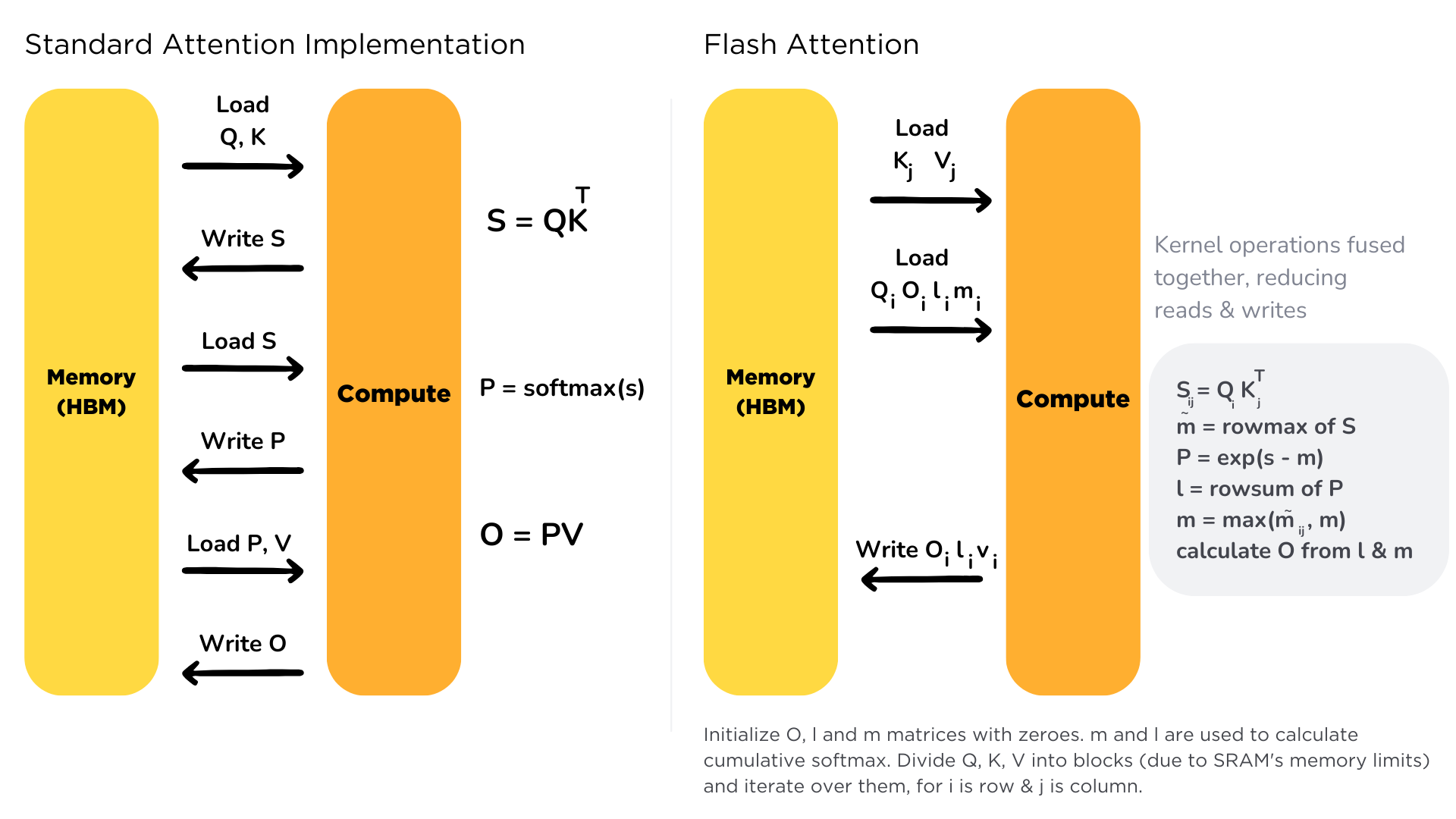
vLLM takes a different approach by using PagedAttention. Just like how a computer manages its memory in pages, vLLM splits the model’s memory into smaller blocks. This clever system means it can handle different-sized requests more flexibly and doesn’t waste memory space. It’s particularly good at sharing memory between different requests and reduces memory fragmentation, which makes the whole system more efficient.
llama.cpp is a highly optimized C/C++ implementation originally designed for running LLaMA models on consumer hardware. It focuses on CPU efficiency with optional GPU acceleration and is ideal for resource-constrained environments. llama.cpp uses quantization techniques to reduce model size and memory requirements while maintaining good performance. It implements optimized kernels for various CPU architectures and supports basic KV cache management for efficient token generation.
Deployment and Integration
Let’s move on to the deployment and integration differences between the frameworks.
TGI excels in enterprise-level deployment with its production-ready features. It comes with built-in Kubernetes support and includes everything you need for running in production, like monitoring through Prometheus and Grafana, automatic scaling, and comprehensive safety features. The system also includes enterprise-grade logging and various protective measures like content filtering and rate limiting to keep your deployment secure and stable.
vLLM takes a more flexible, developer-friendly approach to deployment. It’s built with Python at its core and can easily replace OpenAI’s API in your existing applications. The framework focuses on delivering raw performance and can be customized to fit your specific needs. It works particularly well with Ray for managing clusters, making it a great choice when you need high performance and adaptability.
llama.cpp prioritizes simplicity and portability. Its server implementation is lightweight and can run on a wide range of hardware, from powerful servers to consumer laptops and even some high-end mobile devices. With minimal dependencies and a simple C/C++ core, it’s easy to deploy in environments where installing Python frameworks would be challenging. The server provides an OpenAI-compatible API while maintaining a much smaller resource footprint than other solutions.
Getting Started
Let’s explore how to use these frameworks for deploying LLMs, starting with installation and basic setup.
Installation and Basic Setup
Basic Text Generation
Let’s look at examples of text generation with the frameworks:
Advanced Generation Control
Token Selection and Sampling
The process of generating text involves selecting the next token at each step. This selection process can be controlled through various parameters:
- Raw Logits: The initial output probabilities for each token
- Temperature: Controls randomness in selection (higher = more creative)
- Top-p (Nucleus) Sampling: Filters to top tokens making up X% of probability mass
- Top-k Filtering: Limits selection to k most likely tokens
Here’s how to configure these parameters:
Controlling Repetition
Both frameworks provide ways to prevent repetitive text generation:
Length Control and Stop Sequences
You can control generation length and specify when to stop:
Memory Management
Both frameworks implement advanced memory management techniques for efficient inference.
Resources
- Text Generation Inference Documentation
- TGI GitHub Repository
- vLLM Documentation
- vLLM GitHub Repository
- PagedAttention Paper
- llama.cpp GitHub Repository
- llama-cpp-python Repository
Chapter 3. Fine-tuning a pretrained model
1. Introduction
In Chapter 2 we explored how to use tokenizers and pretrained models to make predictions. But what if you want to fine-tune a pretrained model to solve a specific task? That’s the topic of this chapter! You will learn:
- How to prepare a large dataset from the Hub using the latest 🤗 Datasets features
- How to use the high-level
TrainerAPI to fine-tune a model with modern best practices - How to implement a custom training loop with optimization techniques
- How to leverage the 🤗 Accelerate library to easily run distributed training on any setup
- How to apply current fine-tuning best practices for maximum performance
[!TIP] 📚 Essential Resources: Before starting, you might want to review the 🤗 Datasets documentation for data processing.
This chapter will also serve as an introduction to some Hugging Face libraries beyond the 🤗 Transformers library! We’ll see how libraries like 🤗 Datasets, 🤗 Tokenizers, 🤗 Accelerate, and 🤗 Evaluate can help you train models more efficiently and effectively.
Each of the main sections in this chapter will teach you something different:
- Section 2: Learn modern data preprocessing techniques and efficient dataset handling
- Section 3: Master the powerful Trainer API with all its latest features
- Section 4: Implement training loops from scratch and understand distributed training with Accelerate
By the end of this chapter, you’ll be able to fine-tune models on your own datasets using both high-level APIs and custom training loops, applying the latest best practices in the field.
[!TIP] 🎯 What You’ll Build: By the end of this chapter, you’ll have fine-tuned a BERT model for text classification and understand how to adapt the techniques to your own datasets and tasks.
This chapter focuses exclusively on PyTorch, as it has become the standard framework for modern deep learning research and production. We’ll use the latest APIs and best practices from the Hugging Face ecosystem.
To upload your trained models to the Hugging Face Hub, you will need a Hugging Face account: create an account
2. Processing the data
Continuing with the example from the previous chapter, here is how we would train a sequence classifier on one batch:
import torch
from torch.optim import AdamW
from transformers import AutoTokenizer, AutoModelForSequenceClassification

### Same as before
checkpoint = "bert-base-uncased"
tokenizer = AutoTokenizer.from_pretrained(checkpoint)
model = AutoModelForSequenceClassification.from_pretrained(checkpoint)
sequences = [
    "I've been waiting for a HuggingFace course my whole life.",
    "This course is amazing!",
]
batch = tokenizer(sequences, padding=True, truncation=True, return_tensors="pt")

### This is new
batch["labels"] = torch.tensor([1, 1])

optimizer = AdamW(model.parameters())
loss = model(**batch).loss
loss.backward()
optimizer.step()
Of course, just training the model on two sentences is not going to yield very good results. To get better results, you will need to prepare a bigger dataset.
In this section we will use as an example the MRPC (Microsoft Research Paraphrase Corpus) dataset, introduced in a paper by William B. Dolan and Chris Brockett. The dataset consists of 5,801 pairs of sentences, with a label indicating if they are paraphrases or not (i.e., if both sentences mean the same thing). We’ve selected it for this chapter because it’s a small dataset, so it’s easy to experiment with training on it.
Loading a dataset from the Hub
The Hub doesn’t just contain models; it also has multiple datasets in lots of different languages. You can browse the datasets here, and we recommend you try to load and process a new dataset once you have gone through this section (see the general documentation here). But for now, let’s focus on the MRPC dataset! This is one of the 10 datasets composing the GLUE benchmark, which is an academic benchmark that is used to measure the performance of ML models across 10 different text classification tasks.
The 🤗 Datasets library provides a very simple command to download and cache a dataset on the Hub. We can download the MRPC dataset like this:
[!TIP] 💡 Additional Resources: For more dataset loading techniques and examples, check out the 🤗 Datasets documentation.
from datasets import load_dataset

raw_datasets = load_dataset("glue", "mrpc")
raw_datasets
DatasetDict({
    train: Dataset({
        features: ['sentence1', 'sentence2', 'label', 'idx'],
        num_rows: 3668
    })
    validation: Dataset({
        features: ['sentence1', 'sentence2', 'label', 'idx'],
        num_rows: 408
    })
    test: Dataset({
        features: ['sentence1', 'sentence2', 'label', 'idx'],
        num_rows: 1725
    })
})
As you can see, we get a DatasetDict object which contains the training set, the validation set, and the test set. Each of those contains several columns (sentence1, sentence2, label, and idx) and a variable number of rows, which are the number of elements in each set (so, there are 3,668 pairs of sentences in the training set, 408 in the validation set, and 1,725 in the test set).
[!TIP] This command downloads and caches the dataset, by default in ~/.cache/huggingface/datasets. Recall from Chapter 2 that you can customize your cache folder by setting the
HF_HOMEenvironment variable.
We can access each pair of sentences in our raw_datasets object by indexing, like with a dictionary:
raw_train_dataset = raw_datasets["train"]
raw_train_dataset[0]
{'idx': 0,
 'label': 1,
 'sentence1': 'Amrozi accused his brother , whom he called " the witness " , of deliberately distorting his evidence .',
 'sentence2': 'Referring to him as only " the witness " , Amrozi accused his brother of deliberately distorting his evidence .'}
We can see the labels are already integers, so we won’t have to do any preprocessing there. To know which integer corresponds to which label, we can inspect the features of our raw_train_dataset. This will tell us the type of each column:
raw_train_dataset.features
{'sentence1': Value(dtype='string', id=None),
 'sentence2': Value(dtype='string', id=None),
 'label': ClassLabel(num_classes=2, names=['not_equivalent', 'equivalent'], names_file=None, id=None),
 'idx': Value(dtype='int32', id=None)}
Behind the scenes, label is of type ClassLabel, and the mapping of integers to label name is stored in the names folder. 0 corresponds to not_equivalent, and 1 corresponds to equivalent.
[!TIP] ✏️ Try it out! Look at element 15 of the training set and element 87 of the validation set. What are their labels?
Preprocessing a dataset
To preprocess the dataset, we need to convert the text to numbers the model can make sense of. As you saw in the previous chapter, this is done with a tokenizer. We can feed the tokenizer one sentence or a list of sentences, so we can directly tokenize all the first sentences and all the second sentences of each pair like this:
from transformers import AutoTokenizer

checkpoint = "bert-base-uncased"
tokenizer = AutoTokenizer.from_pretrained(checkpoint)
tokenized_sentences_1 = tokenizer(raw_datasets["train"]["sentence1"])
tokenized_sentences_2 = tokenizer(raw_datasets["train"]["sentence2"])
[!TIP] 💡 Deep Dive: For more advanced tokenization techniques and understanding how different tokenizers work, explore the 🤗 Tokenizers documentation and the tokenization guide in the cookbook.
However, we can’t just pass two sequences to the model and get a prediction of whether the two sentences are paraphrases or not. We need to handle the two sequences as a pair, and apply the appropriate preprocessing. Fortunately, the tokenizer can also take a pair of sequences and prepare it the way our BERT model expects:
inputs = tokenizer("This is the first sentence.", "This is the second one.")
inputs
{
  'input_ids': [101, 2023, 2003, 1996, 2034, 6251, 1012, 102, 2023, 2003, 1996, 2117, 2028, 1012, 102],
  'token_type_ids': [0, 0, 0, 0, 0, 0, 0, 0, 1, 1, 1, 1, 1, 1, 1],
  'attention_mask': [1, 1, 1, 1, 1, 1, 1, 1, 1, 1, 1, 1, 1, 1, 1]
}
We discussed the input_ids and attention_mask keys in Chapter 2, but we put off talking about token_type_ids. In this example, this is what tells the model which part of the input is the first sentence and which is the second sentence.
[!TIP] ✏️ Try it out! Take element 15 of the training set and tokenize the two sentences separately and as a pair. What’s the difference between the two results?
If we decode the IDs inside input_ids back to words:
tokenizer.convert_ids_to_tokens(inputs["input_ids"])
we will get:
['[CLS]', 'this', 'is', 'the', 'first', 'sentence', '.', '[SEP]', 'this', 'is', 'the', 'second', 'one', '.', '[SEP]']
So we see the model expects the inputs to be of the form [CLS] sentence1 [SEP] sentence2 [SEP] when there are two sentences. Aligning this with the token_type_ids gives us:
['[CLS]', 'this', 'is', 'the', 'first', 'sentence', '.', '[SEP]', 'this', 'is', 'the', 'second', 'one', '.', '[SEP]']
[      0,      0,    0,     0,       0,          0,   0,       0,      1,    1,     1,        1,     1,   1,       1]
As you can see, the parts of the input corresponding to [CLS] sentence1 [SEP] all have a token type ID of 0, while the other parts, corresponding to sentence2 [SEP], all have a token type ID of 1.
Note that if you select a different checkpoint, you won’t necessarily have the token_type_ids in your tokenized inputs (for instance, they’re not returned if you use a DistilBERT model). They are only returned when the model will know what to do with them, because it has seen them during its pretraining.
Here, BERT is pretrained with token type IDs, and on top of the masked language modeling objective we talked about in Chapter 1, it has an additional objective called next sentence prediction. The goal with this task is to model the relationship between pairs of sentences.
With next sentence prediction, the model is provided pairs of sentences (with randomly masked tokens) and asked to predict whether the second sentence follows the first. To make the task non-trivial, half of the time the sentences follow each other in the original document they were extracted from, and the other half of the time the two sentences come from two different documents.
In general, you don’t need to worry about whether or not there are token_type_ids in your tokenized inputs: as long as you use the same checkpoint for the tokenizer and the model, everything will be fine as the tokenizer knows what to provide to its model.
Now that we have seen how our tokenizer can deal with one pair of sentences, we can use it to tokenize our whole dataset: like in the previous chapter, we can feed the tokenizer a list of pairs of sentences by giving it the list of first sentences, then the list of second sentences. This is also compatible with the padding and truncation options we saw in Chapter 2. So, one way to preprocess the training dataset is:
tokenized_dataset = tokenizer(
    raw_datasets["train"]["sentence1"],
    raw_datasets["train"]["sentence2"],
    padding=True,
    truncation=True,
)
This works well, but it has the disadvantage of returning a dictionary (with our keys, input_ids, attention_mask, and token_type_ids, and values that are lists of lists). It will also only work if you have enough RAM to store your whole dataset during the tokenization (whereas the datasets from the 🤗 Datasets library are Apache Arrow files stored on the disk, so you only keep the samples you ask for loaded in memory).
To keep the data as a dataset, we will use the Dataset.map() method. This also allows us some extra flexibility, if we need more preprocessing done than just tokenization. The map() method works by applying a function on each element of the dataset, so let’s define a function that tokenizes our inputs:
def tokenize_function(example):
    return tokenizer(example["sentence1"], example["sentence2"], truncation=True)
This function takes a dictionary (like the items of our dataset) and returns a new dictionary with the keys input_ids, attention_mask, and token_type_ids. Note that it also works if the example dictionary contains several samples (each key as a list of sentences) since the tokenizer works on lists of pairs of sentences, as seen before. This will allow us to use the option batched=True in our call to map(), which will greatly speed up the tokenization. The tokenizer is backed by a tokenizer written in Rust from the 🤗 Tokenizers library. This tokenizer can be very fast, but only if we give it lots of inputs at once.
Note that we’ve left the padding argument out in our tokenization function for now. This is because padding all the samples to the maximum length is not efficient: it’s better to pad the samples when we’re building a batch, as then we only need to pad to the maximum length in that batch, and not the maximum length in the entire dataset. This can save a lot of time and processing power when the inputs have very variable lengths!
[!TIP] 📚 Performance Tips: Learn more about efficient data processing techniques in the 🤗 Datasets performance guide.
Here is how we apply the tokenization function on all our datasets at once. We’re using batched=True in our call to map so the function is applied to multiple elements of our dataset at once, and not on each element separately. This allows for faster preprocessing.
tokenized_datasets = raw_datasets.map(tokenize_function, batched=True)
tokenized_datasets
The way the 🤗 Datasets library applies this processing is by adding new fields to the datasets, one for each key in the dictionary returned by the preprocessing function:
DatasetDict({
    train: Dataset({
        features: ['attention_mask', 'idx', 'input_ids', 'label', 'sentence1', 'sentence2', 'token_type_ids'],
        num_rows: 3668
    })
    validation: Dataset({
        features: ['attention_mask', 'idx', 'input_ids', 'label', 'sentence1', 'sentence2', 'token_type_ids'],
        num_rows: 408
    })
    test: Dataset({
        features: ['attention_mask', 'idx', 'input_ids', 'label', 'sentence1', 'sentence2', 'token_type_ids'],
        num_rows: 1725
    })
})
You can even use multiprocessing when applying your preprocessing function with map() by passing along a num_proc argument. We didn’t do this here because the 🤗 Tokenizers library already uses multiple threads to tokenize our samples faster, but if you are not using a fast tokenizer backed by this library, this could speed up your preprocessing.
Our tokenize_function returns a dictionary with the keys input_ids, attention_mask, and token_type_ids, so those three fields are added to all splits of our dataset. Note that we could also have changed existing fields if our preprocessing function returned a new value for an existing key in the dataset to which we applied map().
The last thing we will need to do is pad all the examples to the length of the longest element when we batch elements together — a technique we refer to as dynamic padding.
####### Dynamic padding
The function that is responsible for putting together samples inside a batch is called a collate function. It’s an argument you can pass when you build a DataLoader, the default being a function that will just convert your samples to PyTorch tensors and concatenate them (recursively if your elements are lists, tuples, or dictionaries). This won’t be possible in our case since the inputs we have won’t all be of the same size. We have deliberately postponed the padding, to only apply it as necessary on each batch and avoid having over-long inputs with a lot of padding. This will speed up training by quite a bit, but note that if you’re training on a TPU it can cause problems — TPUs prefer fixed shapes, even when that requires extra padding.
[!TIP] 🚀 Optimization Guide: For more details on optimizing training performance, including padding strategies and TPU considerations, see the 🤗 Transformers performance documentation.
To do this in practice, we have to define a collate function that will apply the correct amount of padding to the items of the dataset we want to batch together. Fortunately, the 🤗 Transformers library provides us with such a function via DataCollatorWithPadding. It takes a tokenizer when you instantiate it (to know which padding token to use, and whether the model expects padding to be on the left or on the right of the inputs) and will do everything you need:
from transformers import DataCollatorWithPadding

data_collator = DataCollatorWithPadding(tokenizer=tokenizer)
To test this new toy, let’s grab a few samples from our training set that we would like to batch together. Here, we remove the columns idx, sentence1, and sentence2 as they won’t be needed and contain strings (and we can’t create tensors with strings) and have a look at the lengths of each entry in the batch:
samples = tokenized_datasets["train"][:8]
samples = {k: v for k, v in samples.items() if k not in ["idx", "sentence1", "sentence2"]}
[len(x) for x in samples["input_ids"]]
[50, 59, 47, 67, 59, 50, 62, 32]
No surprise, we get samples of varying length, from 32 to 67. Dynamic padding means the samples in this batch should all be padded to a length of 67, the maximum length inside the batch. Without dynamic padding, all of the samples would have to be padded to the maximum length in the whole dataset, or the maximum length the model can accept. Let’s double-check that our data_collator is dynamically padding the batch properly:
batch = data_collator(samples)
{k: v.shape for k, v in batch.items()}
{'attention_mask': torch.Size([8, 67]),
 'input_ids': torch.Size([8, 67]),
 'token_type_ids': torch.Size([8, 67]),
 'labels': torch.Size([8])}
Looking good! Now that we’ve gone from raw text to batches our model can deal with, we’re ready to fine-tune it!
[!TIP] ✏️ Try it out! Replicate the preprocessing on the GLUE SST-2 dataset. It’s a little bit different since it’s composed of single sentences instead of pairs, but the rest of what we did should look the same. For a harder challenge, try to write a preprocessing function that works on any of the GLUE tasks.
📖 Additional Practice: Check out these hands-on examples from the 🤗 Transformers examples.
Perfect! Now that we have preprocessed our data with the latest best practices from the 🤗 Datasets library, we’re ready to move on to training our model using the modern Trainer API. The next section will show you how to fine-tune your model effectively using the latest features and optimizations available in the Hugging Face ecosystem.
[!TIP] 💡 Key Takeaways:
- Use
batched=TruewithDataset.map()for significantly faster preprocessing- Dynamic padding with
DataCollatorWithPaddingis more efficient than fixed-length padding- Always preprocess your data to match what your model expects (numerical tensors, correct column names)
- The 🤗 Datasets library provides powerful tools for efficient data processing at scale
3. Fine-tuning a model with the Trainer API
🤗 Transformers provides a Trainer class to help you fine-tune any of the pretrained models it provides on your dataset with modern best practices. Once you’ve done all the data preprocessing work in the last section, you have just a few steps left to define the Trainer. The hardest part is likely to be preparing the environment to run Trainer.train(), as it will run very slowly on a CPU. If you don’t have a GPU set up, you can get access to free GPUs or TPUs on Google Colab.
[!TIP] 📚 Training Resources: Before diving into training, familiarize yourself with the comprehensive 🤗 Transformers training guide and explore practical examples in the fine-tuning cookbook.
The code examples below assume you have already executed the examples in the previous section. Here is a short summary recapping what you need:
from datasets import load_dataset
from transformers import AutoTokenizer, DataCollatorWithPadding

raw_datasets = load_dataset("glue", "mrpc")
checkpoint = "bert-base-uncased"
tokenizer = AutoTokenizer.from_pretrained(checkpoint)


def tokenize_function(example):
    return tokenizer(example["sentence1"], example["sentence2"], truncation=True)


tokenized_datasets = raw_datasets.map(tokenize_function, batched=True)
data_collator = DataCollatorWithPadding(tokenizer=tokenizer)
Training
The first step before we can define our Trainer is to define a TrainingArguments class that will contain all the hyperparameters the Trainer will use for training and evaluation. The only argument you have to provide is a directory where the trained model will be saved, as well as the checkpoints along the way. For all the rest, you can leave the defaults, which should work pretty well for a basic fine-tuning.
from transformers import TrainingArguments

training_args = TrainingArguments("test-trainer")
If you want to automatically upload your model to the Hub during training, pass along push_to_hub=True in the TrainingArguments. We will learn more about this in Chapter 4
[!TIP] 🚀 Advanced Configuration: For detailed information on all available training arguments and optimization strategies, check out the TrainingArguments documentation and the training configuration cookbook.
The second step is to define our model. As in the previous chapter, we will use the AutoModelForSequenceClassification class, with two labels:
from transformers import AutoModelForSequenceClassification

model = AutoModelForSequenceClassification.from_pretrained(checkpoint, num_labels=2)
You will notice that unlike in Chapter 2, you get a warning after instantiating this pretrained model. This is because BERT has not been pretrained on classifying pairs of sentences, so the head of the pretrained model has been discarded and a new head suitable for sequence classification has been added instead. The warnings indicate that some weights were not used (the ones corresponding to the dropped pretraining head) and that some others were randomly initialized (the ones for the new head). It concludes by encouraging you to train the model, which is exactly what we are going to do now.
Once we have our model, we can define a Trainer by passing it all the objects constructed up to now — the model, the training_args, the training and validation datasets, our data_collator, and our processing_class. The processing_class parameter is a newer addition that tells the Trainer which tokenizer to use for processing:
from transformers import Trainer

trainer = Trainer(
    model,
    training_args,
    train_dataset=tokenized_datasets["train"],
    eval_dataset=tokenized_datasets["validation"],
    data_collator=data_collator,
    processing_class=tokenizer,
)
When you pass a tokenizer as the processing_class, the default data_collator used by the Trainer will be a DataCollatorWithPadding. You can skip the data_collator=data_collator line in this case, but we included it here to show you this important part of the processing pipeline.
[!TIP] 📖 Learn More: For comprehensive details on the Trainer class and its parameters, visit the Trainer API documentation and explore advanced usage patterns in the training cookbook recipes.
To fine-tune the model on our dataset, we just have to call the train() method of our Trainer:
trainer.train()
This will start the fine-tuning (which should take a couple of minutes on a GPU) and report the training loss every 500 steps. It won’t, however, tell you how well (or badly) your model is performing. This is because:
- We didn’t tell the
Trainerto evaluate during training by settingeval_strategyinTrainingArgumentsto either"steps"(evaluate everyeval_steps) or"epoch"(evaluate at the end of each epoch). - We didn’t provide the
Trainerwith acompute_metrics()function to calculate a metric during said evaluation (otherwise the evaluation would just have printed the loss, which is not a very intuitive number).
Evaluation
Let’s see how we can build a useful compute_metrics() function and use it the next time we train. The function must take an EvalPrediction object (which is a named tuple with a predictions field and a label_ids field) and will return a dictionary mapping strings to floats (the strings being the names of the metrics returned, and the floats their values). To get some predictions from our model, we can use the Trainer.predict() command:
predictions = trainer.predict(tokenized_datasets["validation"])
print(predictions.predictions.shape, predictions.label_ids.shape)
(408, 2) (408,)
The output of the predict() method is another named tuple with three fields: predictions, label_ids, and metrics. The metrics field will just contain the loss on the dataset passed, as well as some time metrics (how long it took to predict, in total and on average). Once we complete our compute_metrics() function and pass it to the Trainer, that field will also contain the metrics returned by compute_metrics().
As you can see, predictions is a two-dimensional array with shape 408 x 2 (408 being the number of elements in the dataset we used). Those are the logits for each element of the dataset we passed to predict() (as you saw in the previous chapter, all Transformer models return logits). To transform them into predictions that we can compare to our labels, we need to take the index with the maximum value on the second axis:
import numpy as np

preds = np.argmax(predictions.predictions, axis=-1)
We can now compare those preds to the labels. To build our compute_metric() function, we will rely on the metrics from the 🤗 Evaluate library. We can load the metrics associated with the MRPC dataset as easily as we loaded the dataset, this time with the evaluate.load() function. The object returned has a compute() method we can use to do the metric calculation:
import evaluate

metric = evaluate.load("glue", "mrpc")
metric.compute(predictions=preds, references=predictions.label_ids)
{'accuracy': 0.8578431372549019, 'f1': 0.8996539792387542}
[!TIP] Learn about different evaluation metrics and strategies in the 🤗 Evaluate documentation.
The exact results you get may vary, as the random initialization of the model head might change the metrics it achieved. Here, we can see our model has an accuracy of 85.78% on the validation set and an F1 score of 89.97. Those are the two metrics used to evaluate results on the MRPC dataset for the GLUE benchmark. The table in the BERT paper reported an F1 score of 88.9 for the base model. That was the uncased model while we are currently using the cased model, which explains the better result.
Wrapping everything together, we get our compute_metrics() function:
def compute_metrics(eval_preds):
    metric = evaluate.load("glue", "mrpc")
    logits, labels = eval_preds
    predictions = np.argmax(logits, axis=-1)
    return metric.compute(predictions=predictions, references=labels)
And to see it used in action to report metrics at the end of each epoch, here is how we define a new Trainer with this compute_metrics() function:
training_args = TrainingArguments("test-trainer", eval_strategy="epoch")
model = AutoModelForSequenceClassification.from_pretrained(checkpoint, num_labels=2)

trainer = Trainer(
    model,
    training_args,
    train_dataset=tokenized_datasets["train"],
    eval_dataset=tokenized_datasets["validation"],
    data_collator=data_collator,
    processing_class=tokenizer,
    compute_metrics=compute_metrics,
)
Note that we create a new TrainingArguments with its eval_strategy set to "epoch" and a new model — otherwise, we would just be continuing the training of the model we have already trained. To launch a new training run, we execute:
trainer.train()
This time, it will report the validation loss and metrics at the end of each epoch on top of the training loss. Again, the exact accuracy/F1 score you reach might be a bit different from what we found, because of the random head initialization of the model, but it should be in the same ballpark.
Advanced Training Features
The Trainer comes with many built-in features that make modern deep learning best practices accessible:
Mixed Precision Training: Use fp16=True in your training arguments for faster training and reduced memory usage:
training_args = TrainingArguments(
    "test-trainer",
    eval_strategy="epoch",
    fp16=True,  ### Enable mixed precision
)
Gradient Accumulation: For effective larger batch sizes when GPU memory is limited:
training_args = TrainingArguments(
    "test-trainer",
    eval_strategy="epoch",
    per_device_train_batch_size=4,
    gradient_accumulation_steps=4,  ### Effective batch size = 4 * 4 = 16
)
Learning Rate Scheduling: The Trainer uses linear decay by default, but you can customize this:
training_args = TrainingArguments(
    "test-trainer",
    eval_strategy="epoch",
    learning_rate=2e-5,
    lr_scheduler_type="cosine",  ### Try different schedulers
)
[!TIP] 🎯 Performance Optimization: For more advanced training techniques including distributed training, memory optimization, and hardware-specific optimizations, explore the 🤗 Transformers performance guide.
The Trainer will work out of the box on multiple GPUs or TPUs and provides lots of options for distributed training. We will go over everything it supports in Chapter 10.
This concludes the introduction to fine-tuning using the Trainer API. An example of doing this for most common NLP tasks will be given in Chapter 7, but for now let’s look at how to do the same thing with a pure PyTorch training loop.
[!TIP] 📝 More Examples: Check out the comprehensive collection of 🤗 Transformers notebooks. 💡 Key Takeaways:
- The
TrainerAPI provides a high-level interface that handles most training complexity- Use
processing_classto specify your tokenizer for proper data handlingTrainingArgumentscontrols all aspects of training: learning rate, batch size, evaluation strategy, and optimizationscompute_metricsenables custom evaluation metrics beyond just training loss- Modern features like mixed precision (
fp16=True) and gradient accumulation can significantly improve training efficiency
4. A full training loop
Now we’ll see how to achieve the same results as we did in the last section without using the Trainer class, implementing a training loop from scratch with modern PyTorch best practices. Again, we assume you have done the data processing in section 2. Here is a short summary covering everything you will need:
[!TIP] 🏗️ Training from Scratch: This section builds on the previous content. For comprehensive guidance on PyTorch training loops and best practices, check out the 🤗 Transformers training documentation and the custom training cookbook.
from datasets import load_dataset
from transformers import AutoTokenizer, DataCollatorWithPadding

raw_datasets = load_dataset("glue", "mrpc")
checkpoint = "bert-base-uncased"
tokenizer = AutoTokenizer.from_pretrained(checkpoint)


def tokenize_function(example):
    return tokenizer(example["sentence1"], example["sentence2"], truncation=True)


tokenized_datasets = raw_datasets.map(tokenize_function, batched=True)
data_collator = DataCollatorWithPadding(tokenizer=tokenizer)
Prepare for training
Before actually writing our training loop, we will need to define a few objects. The first ones are the dataloaders we will use to iterate over batches. But before we can define those dataloaders, we need to apply a bit of postprocessing to our tokenized_datasets, to take care of some things that the Trainer did for us automatically. Specifically, we need to:
- Remove the columns corresponding to values the model does not expect (like the
sentence1andsentence2columns). - Rename the column
labeltolabels(because the model expects the argument to be namedlabels). - Set the format of the datasets so they return PyTorch tensors instead of lists.
Our tokenized_datasets has one method for each of those steps:
tokenized_datasets = tokenized_datasets.remove_columns(["sentence1", "sentence2", "idx"])
tokenized_datasets = tokenized_datasets.rename_column("label", "labels")
tokenized_datasets.set_format("torch")
tokenized_datasets["train"].column_names
We can then check that the result only has columns that our model will accept:
["attention_mask", "input_ids", "labels", "token_type_ids"]
Now that this is done, we can easily define our dataloaders:
from torch.utils.data import DataLoader

train_dataloader = DataLoader(
    tokenized_datasets["train"], shuffle=True, batch_size=8, collate_fn=data_collator
)
eval_dataloader = DataLoader(
    tokenized_datasets["validation"], batch_size=8, collate_fn=data_collator
)
To quickly check there is no mistake in the data processing, we can inspect a batch like this:
for batch in train_dataloader:
    break
{k: v.shape for k, v in batch.items()}
{'attention_mask': torch.Size([8, 65]),
 'input_ids': torch.Size([8, 65]),
 'labels': torch.Size([8]),
 'token_type_ids': torch.Size([8, 65])}
Note that the actual shapes will probably be slightly different for you since we set shuffle=True for the training dataloader and we are padding to the maximum length inside the batch.
Now that we’re completely finished with data preprocessing (a satisfying yet elusive goal for any ML practitioner), let’s turn to the model. We instantiate it exactly as we did in the previous section:
from transformers import AutoModelForSequenceClassification

model = AutoModelForSequenceClassification.from_pretrained(checkpoint, num_labels=2)
To make sure that everything will go smoothly during training, we pass our batch to this model:
outputs = model(**batch)
print(outputs.loss, outputs.logits.shape)
tensor(0.5441, grad_fn=<NllLossBackward>) torch.Size([8, 2])
All 🤗 Transformers models will return the loss when labels are provided, and we also get the logits (two for each input in our batch, so a tensor of size 8 x 2).
We’re almost ready to write our training loop! We’re just missing two things: an optimizer and a learning rate scheduler. Since we are trying to replicate what the Trainer was doing by hand, we will use the same defaults. The optimizer used by the Trainer is AdamW, which is the same as Adam, but with a twist for weight decay regularization (see “Decoupled Weight Decay Regularization” by Ilya Loshchilov and Frank Hutter):
from torch.optim import AdamW

optimizer = AdamW(model.parameters(), lr=5e-5)
[!TIP] 💡 Modern Optimization Tips: For even better performance, you can try:
- AdamW with weight decay:
AdamW(model.parameters(), lr=5e-5, weight_decay=0.01)- 8-bit Adam: Use
bitsandbytesfor memory-efficient optimization- Different learning rates: Lower learning rates (1e-5 to 3e-5) often work better for large models
🚀 Optimization Resources: Learn more about optimizers and training strategies in the 🤗 Transformers optimization guide.
Finally, the learning rate scheduler used by default is just a linear decay from the maximum value (5e-5) to 0. To properly define it, we need to know the number of training steps we will take, which is the number of epochs we want to run multiplied by the number of training batches (which is the length of our training dataloader). The Trainer uses three epochs by default, so we will follow that:
from transformers import get_scheduler

num_epochs = 3
num_training_steps = num_epochs * len(train_dataloader)
lr_scheduler = get_scheduler(
    "linear",
    optimizer=optimizer,
    num_warmup_steps=0,
    num_training_steps=num_training_steps,
)
print(num_training_steps)
1377
The training loop
One last thing: we will want to use the GPU if we have access to one (on a CPU, training might take several hours instead of a couple of minutes). To do this, we define a device we will put our model and our batches on:
import torch

device = torch.device("cuda") if torch.cuda.is_available() else torch.device("cpu")
model.to(device)
device
device(type='cuda')
We are now ready to train! To get some sense of when training will be finished, we add a progress bar over our number of training steps, using the tqdm library:
from tqdm.auto import tqdm

progress_bar = tqdm(range(num_training_steps))

model.train()
for epoch in range(num_epochs):
    for batch in train_dataloader:
        batch = {k: v.to(device) for k, v in batch.items()}
        outputs = model(**batch)
        loss = outputs.loss
        loss.backward()

        optimizer.step()
        lr_scheduler.step()
        optimizer.zero_grad()
        progress_bar.update(1)
[!TIP] 💡 Modern Training Optimizations: To make your training loop even more efficient, consider:
- Gradient Clipping: Add
torch.nn.utils.clip_grad_norm_(model.parameters(), max_norm=1.0)beforeoptimizer.step()- Mixed Precision: Use
torch.cuda.amp.autocast()andGradScalerfor faster training- Gradient Accumulation: Accumulate gradients over multiple batches to simulate larger batch sizes
- Checkpointing: Save model checkpoints periodically to resume training if interrupted
🔧 Implementation Guide: For detailed examples of these optimizations, see the 🤗 Transformers efficient training guide and the range of optimizers.
You can see that the core of the training loop looks a lot like the one in the introduction. We didn’t ask for any reporting, so this training loop will not tell us anything about how the model fares. We need to add an evaluation loop for that.
The evaluation loop
As we did earlier, we will use a metric provided by the 🤗 Evaluate library. We’ve already seen the metric.compute() method, but metrics can actually accumulate batches for us as we go over the prediction loop with the method add_batch(). Once we have accumulated all the batches, we can get the final result with metric.compute(). Here’s how to implement all of this in an evaluation loop:
[!TIP] 📊 Evaluation Best Practices: For more sophisticated evaluation strategies and metrics, explore the 🤗 Evaluate documentation and the comprehensive evaluation cookbook.
import evaluate

metric = evaluate.load("glue", "mrpc")
model.eval()
for batch in eval_dataloader:
    batch = {k: v.to(device) for k, v in batch.items()}
    with torch.no_grad():
        outputs = model(**batch)

    logits = outputs.logits
    predictions = torch.argmax(logits, dim=-1)
    metric.add_batch(predictions=predictions, references=batch["labels"])

metric.compute()
{'accuracy': 0.8431372549019608, 'f1': 0.8907849829351535}
Again, your results will be slightly different because of the randomness in the model head initialization and the data shuffling, but they should be in the same ballpark.
[!TIP] ✏️ Try it out! Modify the previous training loop to fine-tune your model on the SST-2 dataset.
Supercharge your training loop with 🤗 Accelerate
The training loop we defined earlier works fine on a single CPU or GPU. But using the 🤗 Accelerate library, with just a few adjustments we can enable distributed training on multiple GPUs or TPUs. 🤗 Accelerate handles the complexity of distributed training, mixed precision, and device placement automatically. Starting from the creation of the training and validation dataloaders, here is what our manual training loop looks like:
[!TIP] ⚡ Accelerate Deep Dive: Learn everything about distributed training, mixed precision, and hardware optimization in the 🤗 Accelerate documentation and explore practical examples in the transformers documentation.
from accelerate import Accelerator
from torch.optim import AdamW
from transformers import AutoModelForSequenceClassification, get_scheduler

accelerator = Accelerator()

model = AutoModelForSequenceClassification.from_pretrained(checkpoint, num_labels=2)
optimizer = AdamW(model.parameters(), lr=3e-5)

train_dl, eval_dl, model, optimizer = accelerator.prepare(
    train_dataloader, eval_dataloader, model, optimizer
)

num_epochs = 3
num_training_steps = num_epochs * len(train_dl)
lr_scheduler = get_scheduler(
    "linear",
    optimizer=optimizer,
    num_warmup_steps=0,
    num_training_steps=num_training_steps,
)

progress_bar = tqdm(range(num_training_steps))

model.train()
for epoch in range(num_epochs):
    for batch in train_dl:
        outputs = model(**batch)
        loss = outputs.loss
        accelerator.backward(loss)

        optimizer.step()
        lr_scheduler.step()
        optimizer.zero_grad()
        progress_bar.update(1)
The first line to add is the import line. The second line instantiates an Accelerator object that will look at the environment and initialize the proper distributed setup. 🤗 Accelerate handles the device placement for you, so you can remove the lines that put the model on the device (or, if you prefer, change them to use accelerator.device instead of device).
Then the main bulk of the work is done in the line that sends the dataloaders, the model, and the optimizer to accelerator.prepare(). This will wrap those objects in the proper container to make sure your distributed training works as intended. The remaining changes to make are removing the line that puts the batch on the device (again, if you want to keep this you can just change it to use accelerator.device) and replacing loss.backward() with accelerator.backward(loss).
[!TIP] ⚠️ In order to benefit from the speed-up offered by Cloud TPUs, we recommend padding your samples to a fixed length with the
padding="max_length"andmax_lengtharguments of the tokenizer.
If you’d like to copy and paste it to play around, here’s what the complete training loop looks like with 🤗 Accelerate:
from accelerate import Accelerator
from torch.optim import AdamW
from transformers import AutoModelForSequenceClassification, get_scheduler

accelerator = Accelerator()

model = AutoModelForSequenceClassification.from_pretrained(checkpoint, num_labels=2)
optimizer = AdamW(model.parameters(), lr=3e-5)

train_dl, eval_dl, model, optimizer = accelerator.prepare(
    train_dataloader, eval_dataloader, model, optimizer
)

num_epochs = 3
num_training_steps = num_epochs * len(train_dl)
lr_scheduler = get_scheduler(
    "linear",
    optimizer=optimizer,
    num_warmup_steps=0,
    num_training_steps=num_training_steps,
)

progress_bar = tqdm(range(num_training_steps))

model.train()
for epoch in range(num_epochs):
    for batch in train_dl:
        outputs = model(**batch)
        loss = outputs.loss
        accelerator.backward(loss)

        optimizer.step()
        lr_scheduler.step()
        optimizer.zero_grad()
        progress_bar.update(1)
Putting this in a train.py script will make that script runnable on any kind of distributed setup. To try it out in your distributed setup, run the command:
accelerate config
which will prompt you to answer a few questions and dump your answers in a configuration file used by this command:
accelerate launch train.py
which will launch the distributed training.
If you want to try this in a Notebook (for instance, to test it with TPUs on Colab), just paste the code in a training_function() and run a last cell with:
from accelerate import notebook_launcher

notebook_launcher(training_function)
You can find more examples in the 🤗 Accelerate repo.
[!TIP] 🌐 Distributed Training: For comprehensive coverage of multi-GPU and multi-node training, check out the 🤗 Transformers distributed training guide and the scaling training cookbook.
Next Steps and Best Practices
Now that you’ve learned how to implement training from scratch, here are some additional considerations for production use:
Model Evaluation: Always evaluate your model on multiple metrics, not just accuracy. Use the 🤗 Evaluate library for comprehensive evaluation.
Hyperparameter Tuning: Consider using libraries like Optuna or Ray Tune for systematic hyperparameter optimization.
Model Monitoring: Track training metrics, learning curves, and validation performance throughout training.
Model Sharing: Once trained, share your model on the Hugging Face Hub to make it available to the community.
Efficiency: For large models, consider techniques like gradient checkpointing, parameter-efficient fine-tuning (LoRA, AdaLoRA), or quantization methods.
This concludes our deep dive into fine-tuning with custom training loops. The skills you’ve learned here will serve you well when you need full control over the training process or want to implement custom training logic that goes beyond what the Trainer API offers.
[!TIP] 💡 Key Takeaways:
- Manual training loops give you complete control but require understanding of the proper sequence: forward → backward → optimizer step → scheduler step → zero gradients
- AdamW with weight decay is the recommended optimizer for transformer models
- Always use
model.eval()andtorch.no_grad()during evaluation for correct behavior and efficiency- 🤗 Accelerate makes distributed training accessible with minimal code changes
- Device management (moving tensors to GPU/CPU) is crucial for PyTorch operations
- Modern techniques like mixed precision, gradient accumulation, and gradient clipping can significantly improve training efficiency
5. Understanding Learning Curves
Now that you’ve learned how to implement fine-tuning using both the Trainer API and custom training loops, it’s crucial to understand how to interpret the results. Learning curves are invaluable tools that help you evaluate your model’s performance during training and identify potential issues before they reduce performance.
In this section, we’ll explore how to read and interpret accuracy and loss curves, understand what different curve shapes tell us about our model’s behavior, and learn how to address common training issues.
What are Learning Curves?
Learning curves are visual representations of your model’s performance metrics over time during training. The two most important curves to monitor are:
- Loss curves: Show how the model’s error (loss) changes over training steps or epochs
- Accuracy curves: Show the percentage of correct predictions over training steps or epochs
These curves help us understand whether our model is learning effectively and can guide us in making adjustments to improve performance. In Transformers, these metrics are individually computed for each batch and then logged to the disk. We can then use libraries like Weights & Biases to visualize these curves and track our model’s performance over time.
Loss Curves
The loss curve shows how the model’s error decreases over time. In a typical successful training run, you’ll see a curve similar to the one below:

- High initial loss: The model starts without optimization, so predictions are initially poor
- Decreasing loss: As training progresses, the loss should generally decrease
- Convergence: Eventually, the loss stabilizes at a low value, indicating that the model has learned the patterns in the data
As in previous chapters, we can use the Trainer API to track these metrics and visualize them in a dashboard. Below is an example of how to do this with Weights & Biases.
### Example of tracking loss during training with the Trainer
from transformers import Trainer, TrainingArguments
import wandb

### Initialize Weights & Biases for experiment tracking
wandb.init(project="transformer-fine-tuning", name="bert-mrpc-analysis")

training_args = TrainingArguments(
    output_dir="./results",
    eval_strategy="steps",
    eval_steps=50,
    save_steps=100,
    logging_steps=10,  ### Log metrics every 10 steps
    num_train_epochs=3,
    per_device_train_batch_size=16,
    per_device_eval_batch_size=16,
    report_to="wandb",  ### Send logs to Weights & Biases
)

trainer = Trainer(
    model=model,
    args=training_args,
    train_dataset=tokenized_datasets["train"],
    eval_dataset=tokenized_datasets["validation"],
    data_collator=data_collator,
    processing_class=tokenizer,
    compute_metrics=compute_metrics,
)

### Train and automatically log metrics
trainer.train()
Accuracy Curves
The accuracy curve shows the percentage of correct predictions over time. Unlike loss curves, accuracy curves should generally increase as the model learns and can typically include more steps than the loss curve.

- Start low: Initial accuracy should be low, as the model has not yet learned the patterns in the data
- Increase with training: Accuracy should generally improve as the model learns if it is able to learn the patterns in the data
- May show plateaus: Accuracy often increases in discrete jumps rather than smoothly, as the model makes predictions that are close to the true labels
[!TIP] 💡 Why Accuracy Curves Are “Steppy”: Unlike loss, which is continuous, accuracy is calculated by comparing discrete predictions to true labels. Small improvements in model confidence might not change the final prediction, causing accuracy to remain flat until a threshold is crossed.
Convergence
Convergence occurs when the model’s performance stabilizes and the loss and accuracy curves level off. This is a sign that the model has learned the patterns in the data and is ready to be used. In simple terms, we are aiming for the model to converge to a stable performance every time we train it.

Once models have converged, we can use them to make predictions on new data and refer to evaluation metrics to understand how well the model is performing.
Interpreting Learning Curve Patterns
Different curve shapes reveal different aspects of your model’s training. Let’s examine the most common patterns and what they mean.
Healthy Learning Curves
A well-behaved training run typically shows curve shapes similar to the one below:

Let’s look at the illustration above. It displays both the loss curve (on the left) and the corresponding accuracy curve (on the right). These curves have distinct characteristics.
The loss curve shows the value of the model’s loss over time. Initially, the loss is high and then it gradually decreases, indicating that the model is improving. A decrease in the loss value suggests that the model is making better predictions, as the loss represents the error between the predicted output and the true output.
Now let’s shift our focus to the accuracy curve. It represents the model’s accuracy over time. The accuracy curve begins at a low value and increases as training progresses. Accuracy measures the proportion of correctly classified instances. So, as the accuracy curve rises, it signifies that the model is making more correct predictions.
One notable difference between the curves is the smoothness and the presence of “plateaus” on the accuracy curve. While the loss decreases smoothly, the plateaus on the accuracy curve indicate discrete jumps in accuracy instead of a continuous increase. This behavior is attributed to how accuracy is measured. The loss can improve if the model’s output gets closer to the target, even if the final prediction is still incorrect. Accuracy, however, only improves when the prediction crosses the threshold to be correct.
For example, in a binary classifier distinguishing cats (0) from dogs (1), if the model predicts 0.3 for an image of a dog (true value 1), this is rounded to 0 and is an incorrect classification. If in the next step it predicts 0.4, it’s still incorrect. The loss will have decreased because 0.4 is closer to 1 than 0.3, but the accuracy remains unchanged, creating a plateau. The accuracy will only jump up when the model predicts a value greater than 0.5 that gets rounded to 1.
[!TIP] Characteristics of healthy curves:
- Smooth decline in loss: Both training and validation loss decrease steadily
- Close training/validation performance: Small gap between training and validation metrics
- Convergence: Curves level off, indicating the model has learned the patterns
Practical Examples
Let’s work through some practical examples of learning curves. First, we will highlight some approaches to monitor the learning curves during training. Below, we will break down the different patterns that can be observed in the learning curves.
During Training
During the training process (after you’ve hit trainer.train()), you can monitor these key indicators:
- Loss convergence: Is the loss still decreasing or has it plateaued?
- Overfitting signs: Is validation loss starting to increase while training loss decreases?
- Learning rate: Are the curves too erratic (LR too high) or too flat (LR too low)?
- Stability: Are there sudden spikes or drops that indicate problems?
After Training
After the training process is complete, you can analyze the complete curves to understand the model’s performance.
- Final performance: Did the model reach acceptable performance levels?
- Efficiency: Could the same performance be achieved with fewer epochs?
- Generalization: How close are training and validation performance?
- Trends: Would additional training likely improve performance?
[!TIP] 🔍 W&B Dashboard Features: Weights & Biases automatically creates beautiful, interactive plots of your learning curves. You can:
- Compare multiple runs side by side
- Add custom metrics and visualizations
- Set up alerts for anomalous behavior
- Share results with your team
Learn more in the Weights & Biases documentation.
Overfitting
Overfitting occurs when the model learns too much from the training data and is unable to generalize to different data (represented by the validation set).

Symptoms:
- Training loss continues to decrease while validation loss increases or plateaus
- Large gap between training and validation accuracy
- Training accuracy much higher than validation accuracy
Solutions for overfitting:
- Regularization: Add dropout, weight decay, or other regularization techniques
- Early stopping: Stop training when validation performance stops improving
- Data augmentation: Increase training data diversity
- Reduce model complexity: Use a smaller model or fewer parameters
In the sample below, we use early stopping to prevent overfitting. We set the early_stopping_patience to 3, which means that if the validation loss does not improve for 3 consecutive epochs, the training will be stopped.
### Example of detecting overfitting with early stopping
from transformers import EarlyStoppingCallback

training_args = TrainingArguments(
    output_dir="./results",
    eval_strategy="steps",
    eval_steps=100,
    save_strategy="steps",
    save_steps=100,
    load_best_model_at_end=True,
    metric_for_best_model="eval_loss",
    greater_is_better=False,
    num_train_epochs=10,  ### Set high, but we'll stop early
)

### Add early stopping to prevent overfitting
trainer = Trainer(
    model=model,
    args=training_args,
    train_dataset=tokenized_datasets["train"],
    eval_dataset=tokenized_datasets["validation"],
    data_collator=data_collator,
    processing_class=tokenizer,
    compute_metrics=compute_metrics,
    callbacks=[EarlyStoppingCallback(early_stopping_patience=3)],
)
2. Underfitting
Underfitting occurs when the model is too simple to capture the underlying patterns in the data. This can happen for several reasons:
- The model is too small or lacks capacity to learn the patterns
- The learning rate is too low, causing slow learning
- The dataset is too small or not representative of the problem
- The model is not properly regularized

Symptoms:
- Both training and validation loss remain high
- Model performance plateaus early in training
- Training accuracy is lower than expected
Solutions for underfitting:
- Increase model capacity: Use a larger model or more parameters
- Train longer: Increase the number of epochs
- Adjust learning rate: Try different learning rates
- Check data quality: Ensure your data is properly preprocessed
In the sample below, we train for more epochs to see if the model can learn the patterns in the data.
from transformers import TrainingArguments

training_args = TrainingArguments(
    output_dir="./results",
    -num_train_epochs=5,
    +num_train_epochs=10,
)
3. Erratic Learning Curves
Erratic learning curves occur when the model is not learning effectively. This can happen for several reasons:
- The learning rate is too high, causing the model to overshoot the optimal parameters
- The batch size is too small, causing the model to learn slowly
- The model is not properly regularized, causing it to overfit to the training data
- The dataset is not properly preprocessed, causing the model to learn from noise

Symptoms:
- Frequent fluctuations in loss or accuracy
- Curves show high variance or instability
- Performance oscillates without clear trend
Both training and validation curves show erratic behavior.

Solutions for erratic curves:
- Lower learning rate: Reduce step size for more stable training
- Increase batch size: Larger batches provide more stable gradients
- Gradient clipping: Prevent exploding gradients
- Better data preprocessing: Ensure consistent data quality
In the sample below, we lower the learning rate and increase the batch size.
from transformers import TrainingArguments

training_args = TrainingArguments(
    output_dir="./results",
    -learning_rate=1e-5,
    +learning_rate=1e-4,
    -per_device_train_batch_size=16,
    +per_device_train_batch_size=32,
)
Key Takeaways
Understanding learning curves is crucial for becoming an effective machine learning practitioner. These visual tools provide immediate feedback about your model’s training progress and help you make informed decisions about when to stop training, adjust hyperparameters, or try different approaches. With practice, you’ll develop an intuitive understanding of what healthy learning curves look like and how to address issues when they arise.
[!TIP] 💡 Key Takeaways:
- Learning curves are essential tools for understanding model training progress
- Monitor both loss and accuracy curves, but remember they have different characteristics
- Overfitting shows as diverging training/validation performance
- Underfitting shows as poor performance on both training and validation data
- Tools like Weights & Biases make it easy to track and analyze learning curves
- Early stopping and proper regularization can address most common training issues
🔬 Next Steps: Practice analyzing learning curves on your own fine-tuning experiments. Try different hyperparameters and observe how they affect the curve shapes. This hands-on experience is the best way to develop intuition for reading training progress.
6. Fine-tuning, Check!
That was comprehensive! In the first two chapters you learned about models and tokenizers, and now you know how to fine-tune them for your own data using modern best practices. To recap, in this chapter you:
- Learned about datasets on the Hub and modern data processing techniques
- Learned how to load and preprocess datasets efficiently, including using dynamic padding and data collators
- Implemented fine-tuning and evaluation using the high-level
TrainerAPI with the latest features - Implemented a complete custom training loop from scratch with PyTorch
- Used 🤗 Accelerate to make your training code work seamlessly on multiple GPUs or TPUs
- Applied modern optimization techniques like mixed precision training and gradient accumulation
[!TIP] 🎉 Congratulations! You’ve mastered the fundamentals of fine-tuning transformer models. You’re now ready to tackle real-world ML projects!
📖 Continue Learning: Explore these resources to deepen your knowledge:
- 🤗 Transformers task guides for specific NLP tasks
- 🤗 Transformers examples for comprehensive notebooks
🚀 Next Steps:
- Try fine-tuning on your own dataset using the techniques you’ve learned
- Experiment with different model architectures available on the Hugging Face Hub
- Join the Hugging Face community to share your projects and get help
This is just the beginning of your journey with 🤗 Transformers. In the next chapter, we’ll explore how to share your models and tokenizers with the community and contribute to the ever-growing ecosystem of pretrained models.
The skills you’ve developed here - data preprocessing, training configuration, evaluation, and optimization - are fundamental to any machine learning project. Whether you’re working on text classification, named entity recognition, question answering, or any other NLP task, these techniques will serve you well.
[!TIP] 💡 Pro Tips for Success:
- Always start with a strong baseline using the
TrainerAPI before implementing custom training loops- Use the 🤗 Hub to find pretrained models that are close to your task for better starting points
- Monitor your training with proper evaluation metrics and don’t forget to save checkpoints
- Leverage the community - share your models and datasets to help others and get feedback on your work
Chapter 4. Sharing models and tokenizers
1. The Hugging Face Hub
The Hugging Face Hub –- our main website –- is a central platform that enables anyone to discover, use, and contribute new state-of-the-art models and datasets. It hosts a wide variety of models, with more than 10,000 publicly available. We’ll focus on the models in this chapter, and take a look at the datasets in Chapter 5.
The models in the Hub are not limited to 🤗 Transformers or even NLP. There are models from Flair and AllenNLP for NLP, Asteroid and pyannote for speech, and timm for vision, to name a few.
Each of these models is hosted as a Git repository, which allows versioning and reproducibility. Sharing a model on the Hub means opening it up to the community and making it accessible to anyone looking to easily use it, in turn eliminating their need to train a model on their own and simplifying sharing and usage.
Additionally, sharing a model on the Hub automatically deploys a hosted Inference API for that model. Anyone in the community is free to test it out directly on the model’s page, with custom inputs and appropriate widgets.
The best part is that sharing and using any public model on the Hub is completely free! Paid plans also exist if you wish to share models privately.
The video below shows how to navigate the Hub.
Having a huggingface.co account is required to follow along this part, as we’ll be creating and managing repositories on the Hugging Face Hub: create an account
2. Using pretrained models
The Model Hub makes selecting the appropriate model simple, so that using it in any downstream library can be done in a few lines of code. Let’s take a look at how to actually use one of these models, and how to contribute back to the community.
Let’s say we’re looking for a French-based model that can perform mask filling.
We select the camembert-base checkpoint to try it out. The identifier camembert-base is all we need to start using it! As you’ve seen in previous chapters, we can instantiate it using the pipeline() function:
from transformers import pipeline

camembert_fill_mask = pipeline("fill-mask", model="camembert-base")
results = camembert_fill_mask("Le camembert est <mask> :)")
[
  {'sequence': 'Le camembert est délicieux :)', 'score': 0.49091005325317383, 'token': 7200, 'token_str': 'délicieux'},
  {'sequence': 'Le camembert est excellent :)', 'score': 0.1055697426199913, 'token': 2183, 'token_str': 'excellent'},
  {'sequence': 'Le camembert est succulent :)', 'score': 0.03453313186764717, 'token': 26202, 'token_str': 'succulent'},
  {'sequence': 'Le camembert est meilleur :)', 'score': 0.0330314114689827, 'token': 528, 'token_str': 'meilleur'},
  {'sequence': 'Le camembert est parfait :)', 'score': 0.03007650189101696, 'token': 1654, 'token_str': 'parfait'}
]
As you can see, loading a model within a pipeline is extremely simple. The only thing you need to watch out for is that the chosen checkpoint is suitable for the task it’s going to be used for. For example, here we are loading the camembert-base checkpoint in the fill-mask pipeline, which is completely fine. But if we were to load this checkpoint in the text-classification pipeline, the results would not make any sense because the head of camembert-base is not suitable for this task! We recommend using the task selector in the Hugging Face Hub interface in order to select the appropriate checkpoints:
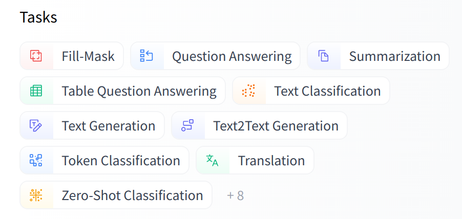
You can also instantiate the checkpoint using the model architecture directly:
from transformers import CamembertTokenizer, CamembertForMaskedLM

tokenizer = CamembertTokenizer.from_pretrained("camembert-base")
model = CamembertForMaskedLM.from_pretrained("camembert-base")
However, we recommend using the Auto* classes instead, as these are by design architecture-agnostic. While the previous code sample limits users to checkpoints loadable in the CamemBERT architecture, using the Auto* classes makes switching checkpoints simple:
from transformers import AutoTokenizer, AutoModelForMaskedLM

tokenizer = AutoTokenizer.from_pretrained("camembert-base")
model = AutoModelForMaskedLM.from_pretrained("camembert-base")
[!TIP] When using a pretrained model, make sure to check how it was trained, on which datasets, its limits, and its biases. All of this information should be indicated on its model card.
3. Sharing pretrained models
In the steps below, we’ll take a look at the easiest ways to share pretrained models to the 🤗 Hub. There are tools and utilities available that make it simple to share and update models directly on the Hub, which we will explore below.
We encourage all users that train models to contribute by sharing them with the community — sharing models, even when trained on very specific datasets, will help others, saving them time and compute resources and providing access to useful trained artifacts. In turn, you can benefit from the work that others have done!
There are three ways to go about creating new model repositories:
- Using the
push_to_hubAPI - Using the
huggingface_hubPython library - Using the web interface
Once you’ve created a repository, you can upload files to it via git and git-lfs. We’ll walk you through creating model repositories and uploading files to them in the following sections.
Using the push_to_hub API
{#if fw === ‘pt’}
{/if}
The simplest way to upload files to the Hub is by leveraging the push_to_hub API.
Before going further, you’ll need to generate an authentication token so that the huggingface_hub API knows who you are and what namespaces you have write access to. Make sure you are in an environment where you have transformers installed (see Setup). If you are in a notebook, you can use the following function to login:
from huggingface_hub import notebook_login

notebook_login()
In a terminal, you can run:
huggingface-cli login
In both cases, you should be prompted for your username and password, which are the same ones you use to log in to the Hub. If you do not have a Hub profile yet, you should create one here.
Great! You now have your authentication token stored in your cache folder. Let’s create some repositories!
If you have played around with the Trainer API to train a model, the easiest way to upload it to the Hub is to set push_to_hub=True when you define your TrainingArguments:
from transformers import TrainingArguments

training_args = TrainingArguments(
    "bert-finetuned-mrpc", save_strategy="epoch", push_to_hub=True
)
When you call trainer.train(), the Trainer will then upload your model to the Hub each time it is saved (here every epoch) in a repository in your namespace. That repository will be named like the output directory you picked (here bert-finetuned-mrpc) but you can choose a different name with hub_model_id = "a_different_name".
To upload your model to an organization you are a member of, just pass it with hub_model_id = "my_organization/my_repo_name".
Once your training is finished, you should do a final trainer.push_to_hub() to upload the last version of your model. It will also generate a model card with all the relevant metadata, reporting the hyperparameters used and the evaluation results! Here is an example of the content you might find in a such a model card:
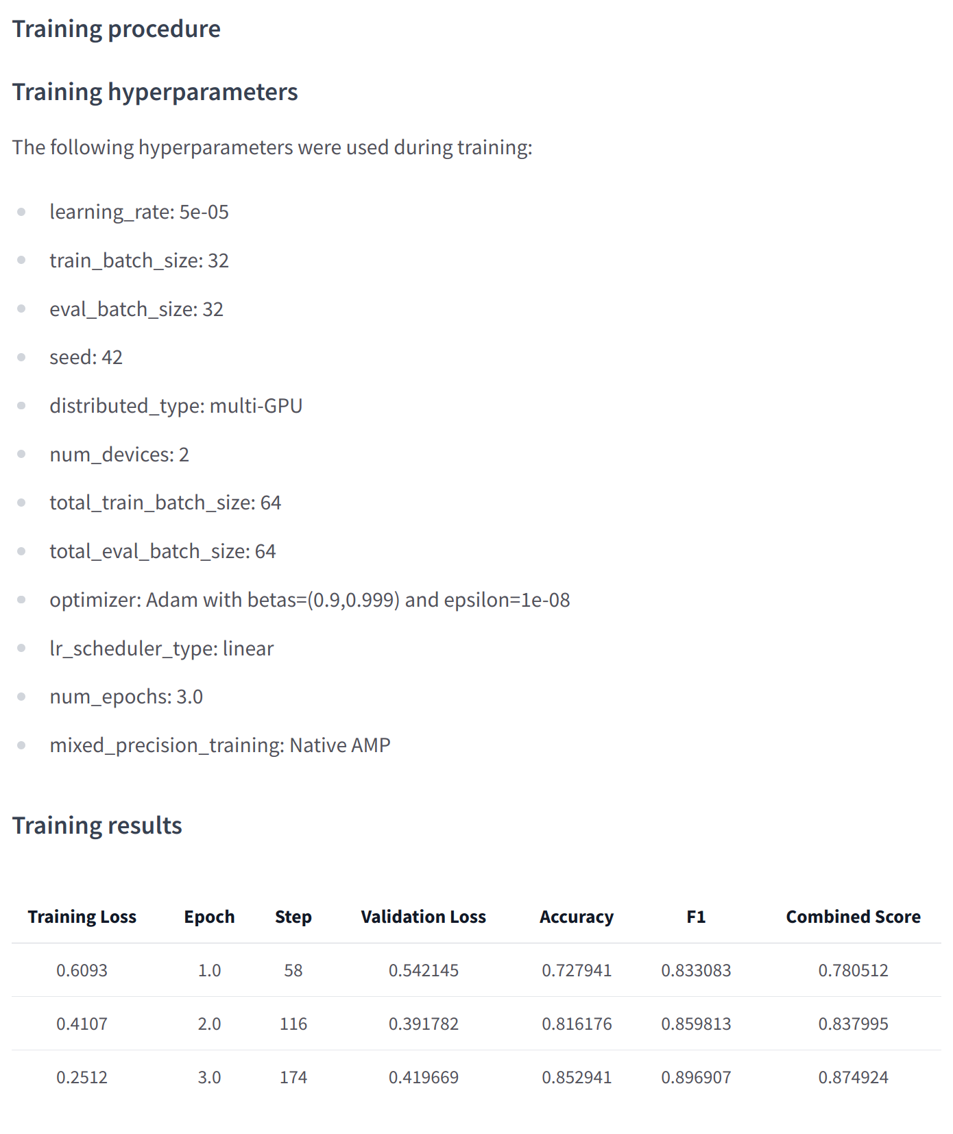
If you are using Keras to train your model, the easiest way to upload it to the Hub is to pass along a PushToHubCallback when you call model.fit():
from transformers import PushToHubCallback

callback = PushToHubCallback(
    "bert-finetuned-mrpc", save_strategy="epoch", tokenizer=tokenizer
)
Then you should add callbacks=[callback] in your call to model.fit(). The callback will then upload your model to the Hub each time it is saved (here every epoch) in a repository in your namespace. That repository will be named like the output directory you picked (here bert-finetuned-mrpc) but you can choose a different name with hub_model_id = "a_different_name".
To upload you model to an organization you are a member of, just pass it with hub_model_id = "my_organization/my_repo_name".
At a lower level, accessing the Model Hub can be done directly on models, tokenizers, and configuration objects via their push_to_hub() method. This method takes care of both the repository creation and pushing the model and tokenizer files directly to the repository. No manual handling is required, unlike with the API we’ll see below.
To get an idea of how it works, let’s first initialize a model and a tokenizer:
from transformers import AutoModelForMaskedLM, AutoTokenizer

checkpoint = "camembert-base"

model = AutoModelForMaskedLM.from_pretrained(checkpoint)
tokenizer = AutoTokenizer.from_pretrained(checkpoint)
You’re free to do whatever you want with these — add tokens to the tokenizer, train the model, fine-tune it. Once you’re happy with the resulting model, weights, and tokenizer, you can leverage the push_to_hub() method directly available on the model object:
model.push_to_hub("dummy-model")
This will create the new repository dummy-model in your profile, and populate it with your model files. Do the same with the tokenizer, so that all the files are now available in this repository:
tokenizer.push_to_hub("dummy-model")
If you belong to an organization, simply specify the organization argument to upload to that organization’s namespace:
tokenizer.push_to_hub("dummy-model", organization="huggingface")
If you wish to use a specific Hugging Face token, you’re free to specify it to the push_to_hub() method as well:
tokenizer.push_to_hub("dummy-model", organization="huggingface", use_auth_token="<TOKEN>")
Now head to the Model Hub to find your newly uploaded model: https://huggingface.co/user-or-organization/dummy-model.
Click on the “Files and versions” tab, and you should see the files visible in the following screenshot:
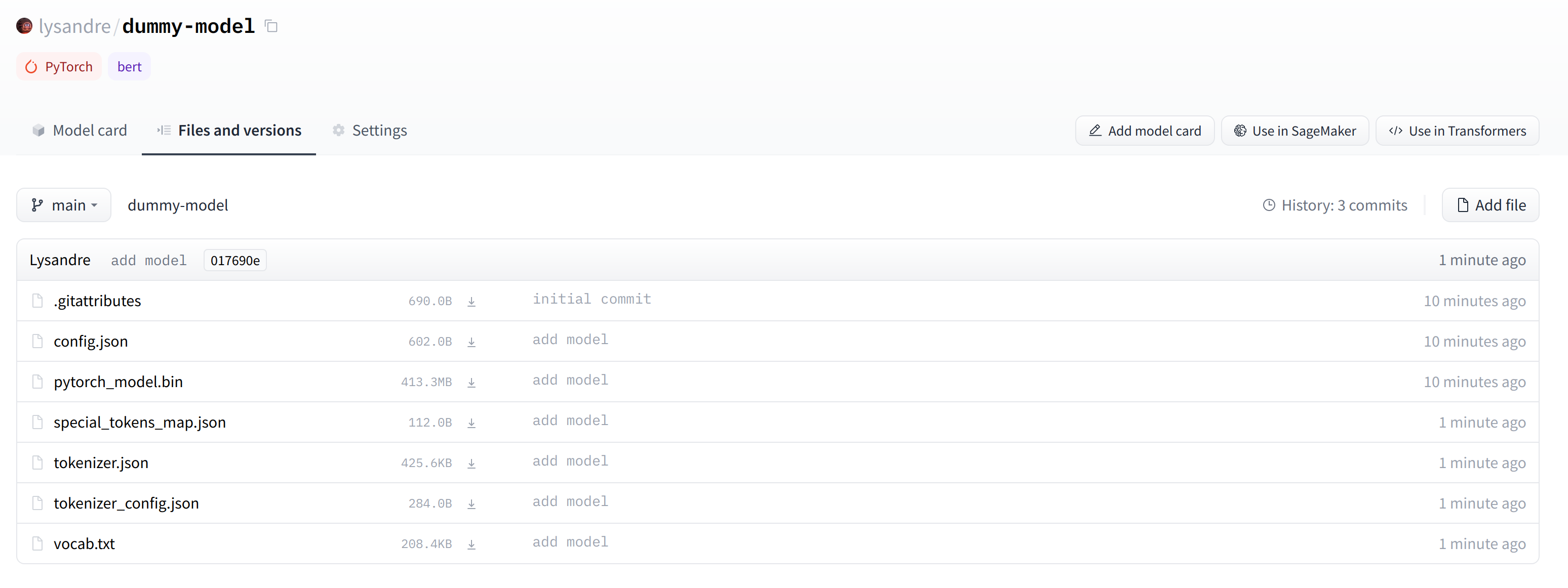
[!TIP] ✏️ Try it out! Take the model and tokenizer associated with the
bert-base-casedcheckpoint and upload them to a repo in your namespace using thepush_to_hub()method. Double-check that the repo appears properly on your page before deleting it.
As you’ve seen, the push_to_hub() method accepts several arguments, making it possible to upload to a specific repository or organization namespace, or to use a different API token. We recommend you take a look at the method specification available directly in the 🤗 Transformers documentation to get an idea of what is possible.
The push_to_hub() method is backed by the huggingface_hub Python package, which offers a direct API to the Hugging Face Hub. It’s integrated within 🤗 Transformers and several other machine learning libraries, like allenlp. Although we focus on the 🤗 Transformers integration in this chapter, integrating it into your own code or library is simple.
Jump to the last section to see how to upload files to your newly created repository!
Using the huggingface_hub Python library
The huggingface_hub Python library is a package which offers a set of tools for the model and datasets hubs. It provides simple methods and classes for common tasks like getting information about repositories on the hub and managing them. It provides simple APIs that work on top of git to manage those repositories’ content and to integrate the Hub in your projects and libraries.
Similarly to using the push_to_hub API, this will require you to have your API token saved in your cache. In order to do this, you will need to use the login command from the CLI, as mentioned in the previous section (again, make sure to prepend these commands with the ! character if running in Google Colab):
huggingface-cli login
The huggingface_hub package offers several methods and classes which are useful for our purpose. Firstly, there are a few methods to manage repository creation, deletion, and others:
```python no-format from huggingface_hub import ( ### User management login, logout, whoami,
### Repository creation and management
create_repo,
delete_repo,
update_repo_visibility,

### And some methods to retrieve/change information about the content
list_models,
list_datasets,
list_metrics,
list_repo_files,
upload_file,
delete_file, ) ```
Additionally, it offers the very powerful Repository class to manage a local repository. We will explore these methods and that class in the next few section to understand how to leverage them.
The create_repo method can be used to create a new repository on the hub:
from huggingface_hub import create_repo

create_repo("dummy-model")
This will create the repository dummy-model in your namespace. If you like, you can specify which organization the repository should belong to using the organization argument:
from huggingface_hub import create_repo

create_repo("dummy-model", organization="huggingface")
This will create the dummy-model repository in the huggingface namespace, assuming you belong to that organization. Other arguments which may be useful are:
private, in order to specify if the repository should be visible from others or not.token, if you would like to override the token stored in your cache by a given token.repo_type, if you would like to create adatasetor aspaceinstead of a model. Accepted values are"dataset"and"space".
Once the repository is created, we should add files to it! Jump to the next section to see the three ways this can be handled.
Using the web interface
The web interface offers tools to manage repositories directly in the Hub. Using the interface, you can easily create repositories, add files (even large ones!), explore models, visualize diffs, and much more.
To create a new repository, visit huggingface.co/new:
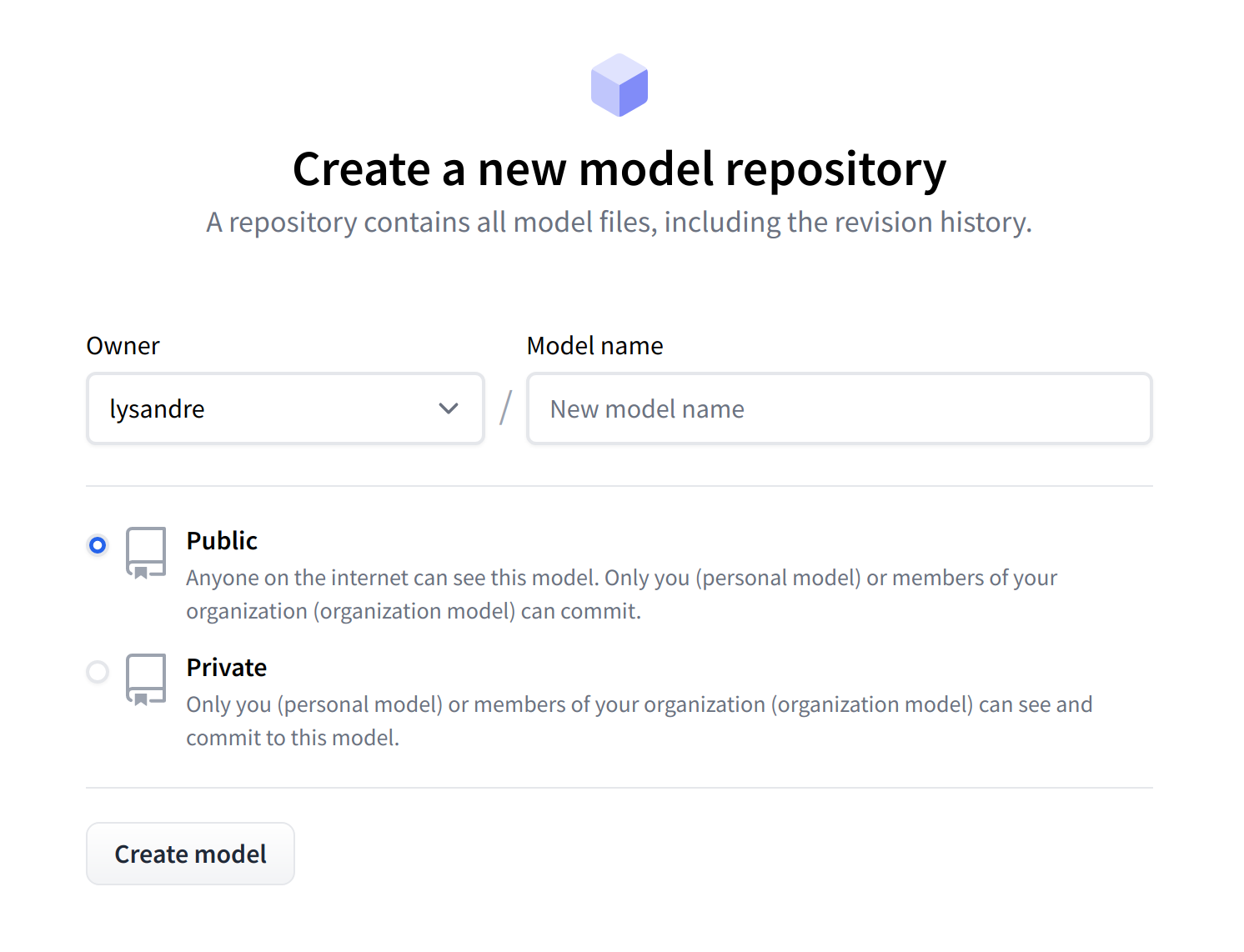
First, specify the owner of the repository: this can be either you or any of the organizations you’re affiliated with. If you choose an organization, the model will be featured on the organization’s page and every member of the organization will have the ability to contribute to the repository.
Next, enter your model’s name. This will also be the name of the repository. Finally, you can specify whether you want your model to be public or private. Private models are hidden from public view.
After creating your model repository, you should see a page like this:
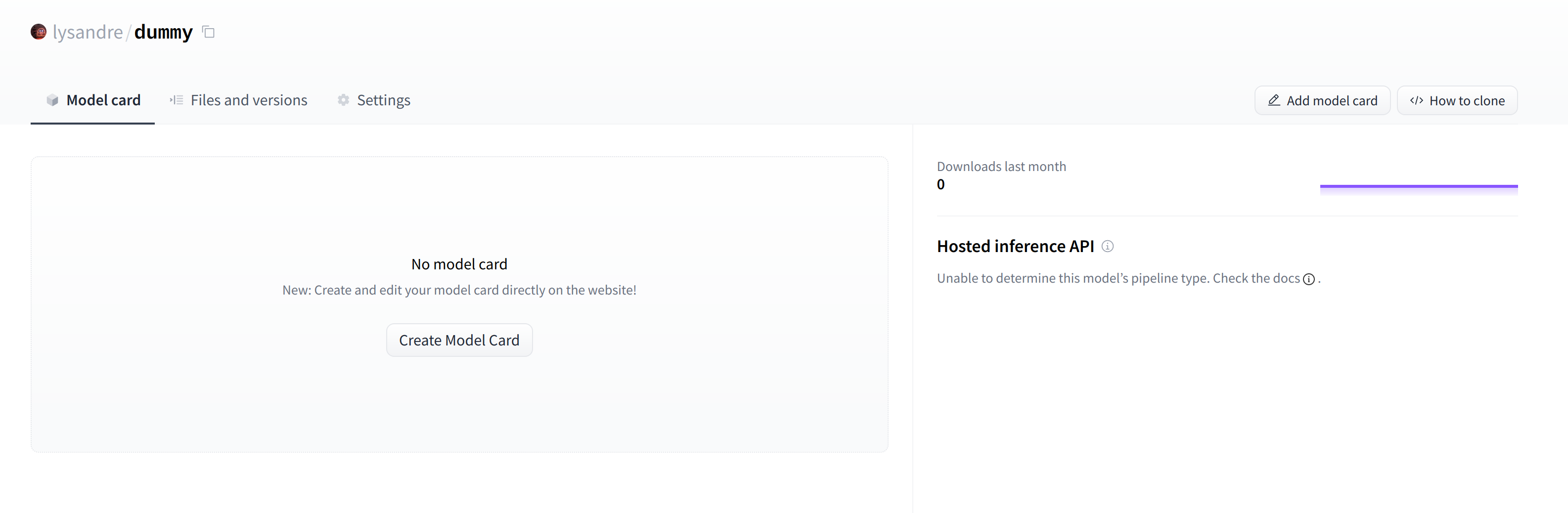
This is where your model will be hosted. To start populating it, you can add a README file directly from the web interface.
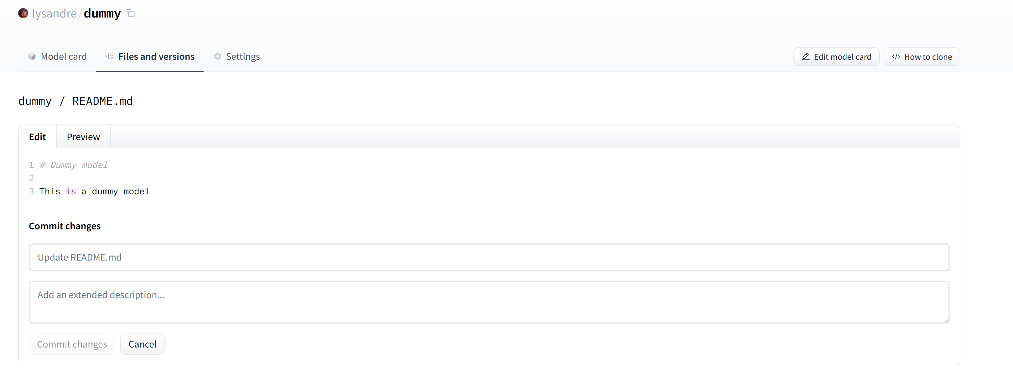
The README file is in Markdown — feel free to go wild with it! The third part of this chapter is dedicated to building a model card. These are of prime importance in bringing value to your model, as they’re where you tell others what it can do.
If you look at the “Files and versions” tab, you’ll see that there aren’t many files there yet — just the README.md you just created and the .gitattributes file that keeps track of large files.
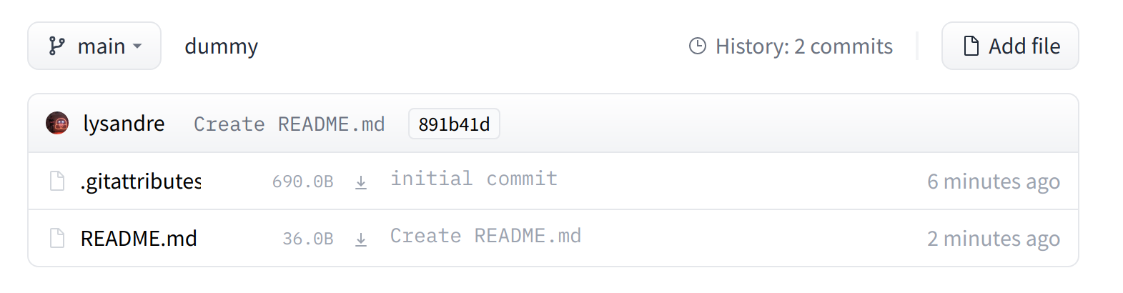
We’ll take a look at how to add some new files next.
Uploading the model files
The system to manage files on the Hugging Face Hub is based on git for regular files, and git-lfs (which stands for Git Large File Storage) for larger files.
In the next section, we go over three different ways of uploading files to the Hub: through huggingface_hub and through git commands.
The upload_file approach
Using upload_file does not require git and git-lfs to be installed on your system. It pushes files directly to the 🤗 Hub using HTTP POST requests. A limitation of this approach is that it doesn’t handle files that are larger than 5GB in size. If your files are larger than 5GB, please follow the two other methods detailed below.
The API may be used as follows:
from huggingface_hub import upload_file

upload_file(
    "<path_to_file>/config.json",
    path_in_repo="config.json",
    repo_id="<namespace>/dummy-model",
)
This will upload the file config.json available at <path_to_file> to the root of the repository as config.json, to the dummy-model repository. Other arguments which may be useful are:
token, if you would like to override the token stored in your cache by a given token.repo_type, if you would like to upload to adatasetor aspaceinstead of a model. Accepted values are"dataset"and"space".
The Repository class
The Repository class manages a local repository in a git-like manner. It abstracts most of the pain points one may have with git to provide all features that we require.
Using this class requires having git and git-lfs installed, so make sure you have git-lfs installed (see here for installation instructions) and set up before you begin.
In order to start playing around with the repository we have just created, we can start by initialising it into a local folder by cloning the remote repository:
from huggingface_hub import Repository

repo = Repository("<path_to_dummy_folder>", clone_from="<namespace>/dummy-model")
This created the folder <path_to_dummy_folder> in our working directory. This folder only contains the .gitattributes file as that’s the only file created when instantiating the repository through create_repo.
From this point on, we may leverage several of the traditional git methods:
repo.git_pull()
repo.git_add()
repo.git_commit()
repo.git_push()
repo.git_tag()
And others! We recommend taking a look at the Repository documentation available here for an overview of all available methods.
At present, we have a model and a tokenizer that we would like to push to the hub. We have successfully cloned the repository, we can therefore save the files within that repository.
We first make sure that our local clone is up to date by pulling the latest changes:
repo.git_pull()
Once that is done, we save the model and tokenizer files:
model.save_pretrained("<path_to_dummy_folder>")
tokenizer.save_pretrained("<path_to_dummy_folder>")
The <path_to_dummy_folder> now contains all the model and tokenizer files. We follow the usual git workflow by adding files to the staging area, committing them and pushing them to the hub:
repo.git_add()
repo.git_commit("Add model and tokenizer files")
repo.git_push()
Congratulations! You just pushed your first files on the hub.
The git-based approach
This is the very barebones approach to uploading files: we’ll do so with git and git-lfs directly. Most of the difficulty is abstracted away by previous approaches, but there are a few caveats with the following method so we’ll follow a more complex use-case.
Using this class requires having git and git-lfs installed, so make sure you have git-lfs installed (see here for installation instructions) and set up before you begin.
First start by initializing git-lfs:
git lfs install
Updated git hooks.
Git LFS initialized.
Once that’s done, the first step is to clone your model repository:
git clone https://huggingface.co/<namespace>/<your-model-id>
My username is lysandre and I’ve used the model name dummy, so for me the command ends up looking like the following:
git clone https://huggingface.co/lysandre/dummy
I now have a folder named dummy in my working directory. I can cd into the folder and have a look at the contents:
cd dummy && ls
README.md
If you just created your repository using Hugging Face Hub’s create_repo method, this folder should only contain a hidden .gitattributes file. If you followed the instructions in the previous section to create a repository using the web interface, the folder should contain a single README.md file alongside the hidden .gitattributes file, as shown here.
Adding a regular-sized file, such as a configuration file, a vocabulary file, or basically any file under a few megabytes, is done exactly as one would do it in any git-based system. However, bigger files must be registered through git-lfs in order to push them to huggingface.co.
Let’s go back to Python for a bit to generate a model and tokenizer that we’d like to commit to our dummy repository:
from transformers import AutoModelForMaskedLM, AutoTokenizer

checkpoint = "camembert-base"

model = AutoModelForMaskedLM.from_pretrained(checkpoint)
tokenizer = AutoTokenizer.from_pretrained(checkpoint)

### Do whatever with the model, train it, fine-tune it...

model.save_pretrained("<path_to_dummy_folder>")
tokenizer.save_pretrained("<path_to_dummy_folder>")
Now that we’ve saved some model and tokenizer artifacts, let’s take another look at the dummy folder:
ls
config.json pytorch_model.bin README.md sentencepiece.bpe.model special_tokens_map.json tokenizer_config.json tokenizer.json
If you look at the file sizes (for example, with ls -lh), you should see that the model state dict file (pytorch_model.bin) is the only outlier, at more than 400 MB.
[!TIP] ✏️ When creating the repository from the web interface, the .gitattributes file is automatically set up to consider files with certain extensions, such as .bin and .h5, as large files, and git-lfs will track them with no necessary setup on your side.
We can now go ahead and proceed like we would usually do with traditional Git repositories. We can add all the files to Git’s staging environment using the git add command:
git add .
We can then have a look at the files that are currently staged:
git status
On branch main
Your branch is up to date with 'origin/main'.

Changes to be committed:
  (use "git restore --staged <file>..." to unstage)
  modified:   .gitattributes
	new file:   config.json
	new file:   pytorch_model.bin
	new file:   sentencepiece.bpe.model
	new file:   special_tokens_map.json
	new file:   tokenizer.json
	new file:   tokenizer_config.json
Similarly, we can make sure that git-lfs is tracking the correct files by using its status command:
git lfs status
On branch main
Objects to be pushed to origin/main:


Objects to be committed:

	config.json (Git: bc20ff2)
	pytorch_model.bin (LFS: 35686c2)
	sentencepiece.bpe.model (LFS: 988bc5a)
	special_tokens_map.json (Git: cb23931)
	tokenizer.json (Git: 851ff3e)
	tokenizer_config.json (Git: f0f7783)

Objects not staged for commit:
We can see that all files have Git as a handler, except pytorch_model.bin and sentencepiece.bpe.model, which have LFS. Great!
Let’s proceed to the final steps, committing and pushing to the huggingface.co remote repository:
git commit -m "First model version"
[main b08aab1] First model version
 7 files changed, 29027 insertions(+)
  6 files changed, 36 insertions(+)
 create mode 100644 config.json
 create mode 100644 pytorch_model.bin
 create mode 100644 sentencepiece.bpe.model
 create mode 100644 special_tokens_map.json
 create mode 100644 tokenizer.json
 create mode 100644 tokenizer_config.json
Pushing can take a bit of time, depending on the speed of your internet connection and the size of your files:
git push
Uploading LFS objects: 100% (1/1), 433 MB | 1.3 MB/s, done.
Enumerating objects: 11, done.
Counting objects: 100% (11/11), done.
Delta compression using up to 12 threads
Compressing objects: 100% (9/9), done.
Writing objects: 100% (9/9), 288.27 KiB | 6.27 MiB/s, done.
Total 9 (delta 1), reused 0 (delta 0), pack-reused 0
To https://huggingface.co/lysandre/dummy
   891b41d..b08aab1  main -> main
If we take a look at the model repository when this is finished, we can see all the recently added files:
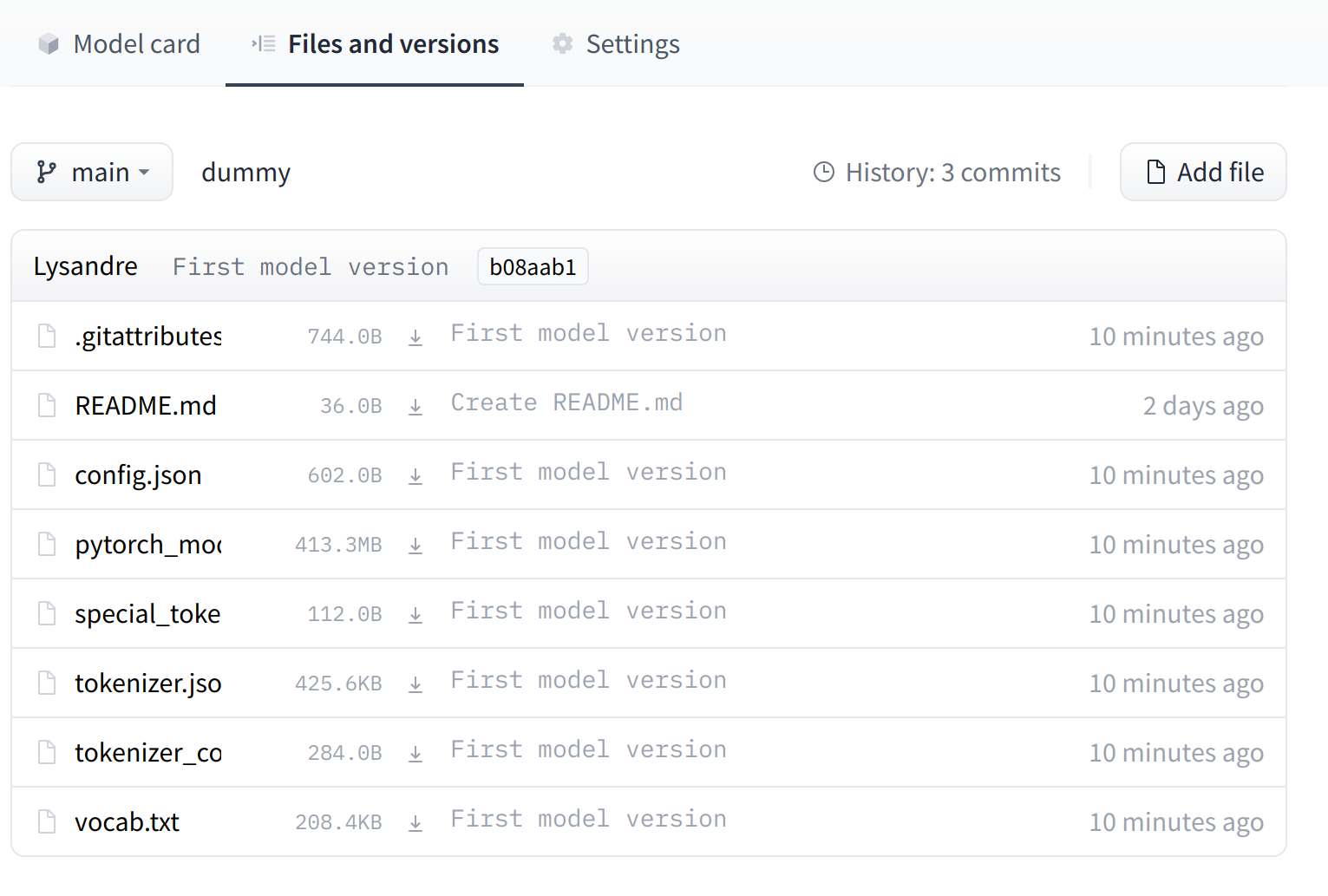
The UI allows you to explore the model files and commits and to see the diff introduced by each commit:
4. Building a model card
The model card is a file which is arguably as important as the model and tokenizer files in a model repository. It is the central definition of the model, ensuring reusability by fellow community members and reproducibility of results, and providing a platform on which other members may build their artifacts.
Documenting the training and evaluation process helps others understand what to expect of a model — and providing sufficient information regarding the data that was used and the preprocessing and postprocessing that were done ensures that the limitations, biases, and contexts in which the model is and is not useful can be identified and understood.
Therefore, creating a model card that clearly defines your model is a very important step. Here, we provide some tips that will help you with this. Creating the model card is done through the README.md file you saw earlier, which is a Markdown file.
The “model card” concept originates from a research direction from Google, first shared in the paper “Model Cards for Model Reporting” by Margaret Mitchell et al. A lot of information contained here is based on that paper, and we recommend you take a look at it to understand why model cards are so important in a world that values reproducibility, reusability, and fairness.
The model card usually starts with a very brief, high-level overview of what the model is for, followed by additional details in the following sections:
- Model description
- Intended uses & limitations
- How to use
- Limitations and bias
- Training data
- Training procedure
- Evaluation results
Let’s take a look at what each of these sections should contain.
Model description
The model description provides basic details about the model. This includes the architecture, version, if it was introduced in a paper, if an original implementation is available, the author, and general information about the model. Any copyright should be attributed here. General information about training procedures, parameters, and important disclaimers can also be mentioned in this section.
Intended uses & limitations
Here you describe the use cases the model is intended for, including the languages, fields, and domains where it can be applied. This section of the model card can also document areas that are known to be out of scope for the model, or where it is likely to perform suboptimally.
How to use
This section should include some examples of how to use the model. This can showcase usage of the pipeline() function, usage of the model and tokenizer classes, and any other code you think might be helpful.
Training data
This part should indicate which dataset(s) the model was trained on. A brief description of the dataset(s) is also welcome.
Training procedure
In this section you should describe all the relevant aspects of training that are useful from a reproducibility perspective. This includes any preprocessing and postprocessing that were done on the data, as well as details such as the number of epochs the model was trained for, the batch size, the learning rate, and so on.
Variable and metrics
Here you should describe the metrics you use for evaluation, and the different factors you are mesuring. Mentioning which metric(s) were used, on which dataset and which dataset split, makes it easy to compare you model’s performance compared to that of other models. These should be informed by the previous sections, such as the intended users and use cases.
Evaluation results
Finally, provide an indication of how well the model performs on the evaluation dataset. If the model uses a decision threshold, either provide the decision threshold used in the evaluation, or provide details on evaluation at different thresholds for the intended uses.
Example
Check out the following for a few examples of well-crafted model cards:
More examples from different organizations and companies are available here.
Note
Model cards are not a requirement when publishing models, and you don’t need to include all of the sections described above when you make one. However, explicit documentation of the model can only benefit future users, so we recommend that you fill in as many of the sections as possible to the best of your knowledge and ability.
Model card metadata
If you have done a little exploring of the Hugging Face Hub, you should have seen that some models belong to certain categories: you can filter them by tasks, languages, libraries, and more. The categories a model belongs to are identified according to the metadata you add in the model card header.
For example, if you take a look at the camembert-base model card, you should see the following lines in the model card header:
---
language: fr
license: mit
datasets:
- oscar
---
This metadata is parsed by the Hugging Face Hub, which then identifies this model as being a French model, with an MIT license, trained on the Oscar dataset.
The full model card specification allows specifying languages, licenses, tags, datasets, metrics, as well as the evaluation results the model obtained when training.
Chapter 5. The 🤗 Datasets library
1. Introduction
In Chapter 3 you got your first taste of the 🤗 Datasets library and saw that there were three main steps when it came to fine-tuning a model:
- Load a dataset from the Hugging Face Hub.
- Preprocess the data with
Dataset.map(). - Load and compute metrics.
But this is just scratching the surface of what 🤗 Datasets can do! In this chapter, we will take a deep dive into the library. Along the way, we’ll find answers to the following questions:
- What do you do when your dataset is not on the Hub?
- How can you slice and dice a dataset? (And what if you really need to use Pandas?)
- What do you do when your dataset is huge and will melt your laptop’s RAM?
- What the heck are “memory mapping” and Apache Arrow?
- How can you create your own dataset and push it to the Hub?
The techniques you learn here will prepare you for the advanced tokenization and fine-tuning tasks in Chapter 6 and Chapter 7 – so grab a coffee and let’s get started!
2. What if my dataset isn’t on the Hub?
You know how to use the Hugging Face Hub to download datasets, but you’ll often find yourself working with data that is stored either on your laptop or on a remote server. In this section we’ll show you how 🤗 Datasets can be used to load datasets that aren’t available on the Hugging Face Hub.
Working with local and remote datasets
🤗 Datasets provides loading scripts to handle the loading of local and remote datasets. It supports several common data formats, such as:
| Data format | Loading script | Example |
|---|---|---|
| CSV & TSV | csv | load_dataset("csv", data_files="my_file.csv") |
| Text files | text | load_dataset("text", data_files="my_file.txt") |
| JSON & JSON Lines | json | load_dataset("json", data_files="my_file.jsonl") |
| Pickled DataFrames | pandas | load_dataset("pandas", data_files="my_dataframe.pkl") |
As shown in the table, for each data format we just need to specify the type of loading script in the load_dataset() function, along with a data_files argument that specifies the path to one or more files. Let’s start by loading a dataset from local files; later we’ll see how to do the same with remote files.
Loading a local dataset
For this example we’ll use the SQuAD-it dataset, which is a large-scale dataset for question answering in Italian.
The training and test splits are hosted on GitHub, so we can download them with a simple wget command:
!wget https://github.com/crux82/squad-it/raw/master/SQuAD_it-train.json.gz
!wget https://github.com/crux82/squad-it/raw/master/SQuAD_it-test.json.gz
This will download two compressed files called SQuAD_it-train.json.gz and SQuAD_it-test.json.gz, which we can decompress with the Linux gzip command:
!gzip -dkv SQuAD_it-*.json.gz
SQuAD_it-test.json.gz:	   87.4% -- replaced with SQuAD_it-test.json
SQuAD_it-train.json.gz:	   82.2% -- replaced with SQuAD_it-train.json
We can see that the compressed files have been replaced with SQuAD_it-train.json and SQuAD_it-test.json, and that the data is stored in the JSON format.
[!TIP] ✎ If you’re wondering why there’s a
!character in the above shell commands, that’s because we’re running them within a Jupyter notebook. Simply remove the prefix if you want to download and unzip the dataset within a terminal.
To load a JSON file with the load_dataset() function, we just need to know if we’re dealing with ordinary JSON (similar to a nested dictionary) or JSON Lines (line-separated JSON). Like many question answering datasets, SQuAD-it uses the nested format, with all the text stored in a data field. This means we can load the dataset by specifying the field argument as follows:
from datasets import load_dataset

squad_it_dataset = load_dataset("json", data_files="SQuAD_it-train.json", field="data")
By default, loading local files creates a DatasetDict object with a train split. We can see this by inspecting the squad_it_dataset object:
squad_it_dataset
DatasetDict({
    train: Dataset({
        features: ['title', 'paragraphs'],
        num_rows: 442
    })
})
This shows us the number of rows and the column names associated with the training set. We can view one of the examples by indexing into the train split as follows:
squad_it_dataset["train"][0]
{
    "title": "Terremoto del Sichuan del 2008",
    "paragraphs": [
        {
            "context": "Il terremoto del Sichuan del 2008 o il terremoto...",
            "qas": [
                {
                    "answers": [{"answer_start": 29, "text": "2008"}],
                    "id": "56cdca7862d2951400fa6826",
                    "question": "In quale anno si è verificato il terremoto nel Sichuan?",
                },
                ...
            ],
        },
        ...
    ],
}
Great, we’ve loaded our first local dataset! But while this worked for the training set, what we really want is to include both the train and test splits in a single DatasetDict object so we can apply Dataset.map() functions across both splits at once. To do this, we can provide a dictionary to the data_files argument that maps each split name to a file associated with that split:
data_files = {"train": "SQuAD_it-train.json", "test": "SQuAD_it-test.json"}
squad_it_dataset = load_dataset("json", data_files=data_files, field="data")
squad_it_dataset
DatasetDict({
    train: Dataset({
        features: ['title', 'paragraphs'],
        num_rows: 442
    })
    test: Dataset({
        features: ['title', 'paragraphs'],
        num_rows: 48
    })
})
This is exactly what we wanted. Now, we can apply various preprocessing techniques to clean up the data, tokenize the reviews, and so on.
[!TIP] The
data_filesargument of theload_dataset()function is quite flexible and can be either a single file path, a list of file paths, or a dictionary that maps split names to file paths. You can also glob files that match a specified pattern according to the rules used by the Unix shell (e.g., you can glob all the JSON files in a directory as a single split by settingdata_files="*.json"). See the 🤗 Datasets documentation for more details.
The loading scripts in 🤗 Datasets actually support automatic decompression of the input files, so we could have skipped the use of gzip by pointing the data_files argument directly to the compressed files:
data_files = {"train": "SQuAD_it-train.json.gz", "test": "SQuAD_it-test.json.gz"}
squad_it_dataset = load_dataset("json", data_files=data_files, field="data")
This can be useful if you don’t want to manually decompress many GZIP files. The automatic decompression also applies to other common formats like ZIP and TAR, so you just need to point data_files to the compressed files and you’re good to go!
Now that you know how to load local files on your laptop or desktop, let’s take a look at loading remote files.
Loading a remote dataset
If you’re working as a data scientist or coder in a company, there’s a good chance the datasets you want to analyze are stored on some remote server. Fortunately, loading remote files is just as simple as loading local ones! Instead of providing a path to local files, we point the data_files argument of load_dataset() to one or more URLs where the remote files are stored. For example, for the SQuAD-it dataset hosted on GitHub, we can just point data_files to the SQuAD_it-*.json.gz URLs as follows:
url = "https://github.com/crux82/squad-it/raw/master/"
data_files = {
    "train": url + "SQuAD_it-train.json.gz",
    "test": url + "SQuAD_it-test.json.gz",
}
squad_it_dataset = load_dataset("json", data_files=data_files, field="data")
This returns the same DatasetDict object obtained above, but saves us the step of manually downloading and decompressing the SQuAD_it-*.json.gz files. This wraps up our foray into the various ways to load datasets that aren’t hosted on the Hugging Face Hub. Now that we’ve got a dataset to play with, let’s get our hands dirty with various data-wrangling techniques!
[!TIP] ✏️ Try it out! Pick another dataset hosted on GitHub or the UCI Machine Learning Repository and try loading it both locally and remotely using the techniques introduced above. For bonus points, try loading a dataset that’s stored in a CSV or text format (see the documentation for more information on these formats).
3. Time to slice and dice
Most of the time, the data you work with won’t be perfectly prepared for training models. In this section we’ll explore the various features that 🤗 Datasets provides to clean up your datasets.
Slicing and dicing our data
Similar to Pandas, 🤗 Datasets provides several functions to manipulate the contents of Dataset and DatasetDict objects. We already encountered the Dataset.map() method in Chapter 3, and in this section we’ll explore some of the other functions at our disposal.
For this example we’ll use the Drug Review Dataset that’s hosted on the UC Irvine Machine Learning Repository, which contains patient reviews on various drugs, along with the condition being treated and a 10-star rating of the patient’s satisfaction.
First we need to download and extract the data, which can be done with the wget and unzip commands:
!wget "https://archive.ics.uci.edu/ml/machine-learning-databases/00462/drugsCom_raw.zip"
!unzip drugsCom_raw.zip
Since TSV is just a variant of CSV that uses tabs instead of commas as the separator, we can load these files by using the csv loading script and specifying the delimiter argument in the load_dataset() function as follows:
from datasets import load_dataset

data_files = {"train": "drugsComTrain_raw.tsv", "test": "drugsComTest_raw.tsv"}
### \t is the tab character in Python
drug_dataset = load_dataset("csv", data_files=data_files, delimiter="\t")
A good practice when doing any sort of data analysis is to grab a small random sample to get a quick feel for the type of data you’re working with. In 🤗 Datasets, we can create a random sample by chaining the Dataset.shuffle() and Dataset.select() functions together:
drug_sample = drug_dataset["train"].shuffle(seed=42).select(range(1000))
### Peek at the first few examples
drug_sample[:3]
{'Unnamed: 0': [87571, 178045, 80482],
 'drugName': ['Naproxen', 'Duloxetine', 'Mobic'],
 'condition': ['Gout, Acute', 'ibromyalgia', 'Inflammatory Conditions'],
 'review': ['"like the previous person mention, I'm a strong believer of aleve, it works faster for my gout than the prescription meds I take. No more going to the doctor for refills.....Aleve works!"',
  '"I have taken Cymbalta for about a year and a half for fibromyalgia pain. It is great\r\nas a pain reducer and an anti-depressant, however, the side effects outweighed \r\nany benefit I got from it. I had trouble with restlessness, being tired constantly,\r\ndizziness, dry mouth, numbness and tingling in my feet, and horrible sweating. I am\r\nbeing weaned off of it now. Went from 60 mg to 30mg and now to 15 mg. I will be\r\noff completely in about a week. The fibro pain is coming back, but I would rather deal with it than the side effects."',
  '"I have been taking Mobic for over a year with no side effects other than an elevated blood pressure.  I had severe knee and ankle pain which completely went away after taking Mobic.  I attempted to stop the medication however pain returned after a few days."'],
 'rating': [9.0, 3.0, 10.0],
 'date': ['September 2, 2015', 'November 7, 2011', 'June 5, 2013'],
 'usefulCount': [36, 13, 128]}
Note that we’ve fixed the seed in Dataset.shuffle() for reproducibility purposes. Dataset.select() expects an iterable of indices, so we’ve passed range(1000) to grab the first 1,000 examples from the shuffled dataset. From this sample we can already see a few quirks in our dataset:
- The
Unnamed: 0column looks suspiciously like an anonymized ID for each patient. - The
conditioncolumn includes a mix of uppercase and lowercase labels. - The reviews are of varying length and contain a mix of Python line separators (
\r\n) as well as HTML character codes like&\#039;.
Let’s see how we can use 🤗 Datasets to deal with each of these issues. To test the patient ID hypothesis for the Unnamed: 0 column, we can use the Dataset.unique() function to verify that the number of IDs matches the number of rows in each split:
for split in drug_dataset.keys():
    assert len(drug_dataset[split]) == len(drug_dataset[split].unique("Unnamed: 0"))
This seems to confirm our hypothesis, so let’s clean up the dataset a bit by renaming the Unnamed: 0 column to something a bit more interpretable. We can use the DatasetDict.rename_column() function to rename the column across both splits in one go:
drug_dataset = drug_dataset.rename_column(
    original_column_name="Unnamed: 0", new_column_name="patient_id"
)
drug_dataset
DatasetDict({
    train: Dataset({
        features: ['patient_id', 'drugName', 'condition', 'review', 'rating', 'date', 'usefulCount'],
        num_rows: 161297
    })
    test: Dataset({
        features: ['patient_id', 'drugName', 'condition', 'review', 'rating', 'date', 'usefulCount'],
        num_rows: 53766
    })
})
[!TIP] ✏️ Try it out! Use the
Dataset.unique()function to find the number of unique drugs and conditions in the training and test sets.
Next, let’s normalize all the condition labels using Dataset.map(). As we did with tokenization in Chapter 3, we can define a simple function that can be applied across all the rows of each split in drug_dataset:
def lowercase_condition(example):
    return {"condition": example["condition"].lower()}


drug_dataset.map(lowercase_condition)
AttributeError: 'NoneType' object has no attribute 'lower'
Oh no, we’ve run into a problem with our map function! From the error we can infer that some of the entries in the condition column are None, which cannot be lowercased as they’re not strings. Let’s drop these rows using Dataset.filter(), which works in a similar way to Dataset.map() and expects a function that receives a single example of the dataset. Instead of writing an explicit function like:
def filter_nones(x):
    return x["condition"] is not None
and then running drug_dataset.filter(filter_nones), we can do this in one line using a lambda function. In Python, lambda functions are small functions that you can define without explicitly naming them. They take the general form:
lambda <arguments> : <expression>
where lambda is one of Python’s special keywords, <arguments> is a list/set of comma-separated values that define the inputs to the function, and <expression> represents the operations you wish to execute. For example, we can define a simple lambda function that squares a number as follows:
lambda x : x * x
To apply this function to an input, we need to wrap it and the input in parentheses:
(lambda x: x * x)(3)
9
Similarly, we can define lambda functions with multiple arguments by separating them with commas. For example, we can compute the area of a triangle as follows:
(lambda base, height: 0.5 * base * height)(4, 8)
16.0
Lambda functions are handy when you want to define small, single-use functions (for more information about them, we recommend reading the excellent Real Python tutorial by Andre Burgaud). In the 🤗 Datasets context, we can use lambda functions to define simple map and filter operations, so let’s use this trick to eliminate the None entries in our dataset:
drug_dataset = drug_dataset.filter(lambda x: x["condition"] is not None)
With the None entries removed, we can normalize our condition column:
drug_dataset = drug_dataset.map(lowercase_condition)
### Check that lowercasing worked
drug_dataset["train"]["condition"][:3]
['left ventricular dysfunction', 'adhd', 'birth control']
It works! Now that we’ve cleaned up the labels, let’s take a look at cleaning up the reviews themselves.
Creating new columns
Whenever you’re dealing with customer reviews, a good practice is to check the number of words in each review. A review might be just a single word like “Great!” or a full-blown essay with thousands of words, and depending on the use case you’ll need to handle these extremes differently. To compute the number of words in each review, we’ll use a rough heuristic based on splitting each text by whitespace.
Let’s define a simple function that counts the number of words in each review:
def compute_review_length(example):
    return {"review_length": len(example["review"].split())}
Unlike our lowercase_condition() function, compute_review_length() returns a dictionary whose key does not correspond to one of the column names in the dataset. In this case, when compute_review_length() is passed to Dataset.map(), it will be applied to all the rows in the dataset to create a new review_length column:
drug_dataset = drug_dataset.map(compute_review_length)
### Inspect the first training example
drug_dataset["train"][0]
{'patient_id': 206461,
 'drugName': 'Valsartan',
 'condition': 'left ventricular dysfunction',
 'review': '"It has no side effect, I take it in combination of Bystolic 5 Mg and Fish Oil"',
 'rating': 9.0,
 'date': 'May 20, 2012',
 'usefulCount': 27,
 'review_length': 17}
As expected, we can see a review_length column has been added to our training set. We can sort this new column with Dataset.sort() to see what the extreme values look like:
drug_dataset["train"].sort("review_length")[:3]
{'patient_id': [103488, 23627, 20558],
 'drugName': ['Loestrin 21 1 / 20', 'Chlorzoxazone', 'Nucynta'],
 'condition': ['birth control', 'muscle spasm', 'pain'],
 'review': ['"Excellent."', '"useless"', '"ok"'],
 'rating': [10.0, 1.0, 6.0],
 'date': ['November 4, 2008', 'March 24, 2017', 'August 20, 2016'],
 'usefulCount': [5, 2, 10],
 'review_length': [1, 1, 1]}
As we suspected, some reviews contain just a single word, which, although it may be okay for sentiment analysis, would not be informative if we want to predict the condition.
[!TIP] 🙋 An alternative way to add new columns to a dataset is with the
Dataset.add_column()function. This allows you to provide the column as a Python list or NumPy array and can be handy in situations whereDataset.map()is not well suited for your analysis.
Let’s use the Dataset.filter() function to remove reviews that contain fewer than 30 words. Similarly to what we did with the condition column, we can filter out the very short reviews by requiring that the reviews have a length above this threshold:
drug_dataset = drug_dataset.filter(lambda x: x["review_length"] > 30)
print(drug_dataset.num_rows)
{'train': 138514, 'test': 46108}
As you can see, this has removed around 15% of the reviews from our original training and test sets.
[!TIP] ✏️ Try it out! Use the
Dataset.sort()function to inspect the reviews with the largest numbers of words. See the documentation to see which argument you need to use sort the reviews by length in descending order.
The last thing we need to deal with is the presence of HTML character codes in our reviews. We can use Python’s html module to unescape these characters, like so:
import html

text = "I'm a transformer called BERT"
html.unescape(text)
"I'm a transformer called BERT"
We’ll use Dataset.map() to unescape all the HTML characters in our corpus:
drug_dataset = drug_dataset.map(lambda x: {"review": html.unescape(x["review"])})
As you can see, the Dataset.map() method is quite useful for processing data – and we haven’t even scratched the surface of everything it can do!
The map() method’s superpowers
The Dataset.map() method takes a batched argument that, if set to True, causes it to send a batch of examples to the map function at once (the batch size is configurable but defaults to 1,000). For instance, the previous map function that unescaped all the HTML took a bit of time to run (you can read the time taken from the progress bars). We can speed this up by processing several elements at the same time using a list comprehension.
When you specify batched=True the function receives a dictionary with the fields of the dataset, but each value is now a list of values, and not just a single value. The return value of Dataset.map() should be the same: a dictionary with the fields we want to update or add to our dataset, and a list of values. For example, here is another way to unescape all HTML characters, but using batched=True:
new_drug_dataset = drug_dataset.map(
    lambda x: {"review": [html.unescape(o) for o in x["review"]]}, batched=True
)
If you’re running this code in a notebook, you’ll see that this command executes way faster than the previous one. And it’s not because our reviews have already been HTML-unescaped – if you re-execute the instruction from the previous section (without batched=True), it will take the same amount of time as before. This is because list comprehensions are usually faster than executing the same code in a for loop, and we also gain some performance by accessing lots of elements at the same time instead of one by one.
Using Dataset.map() with batched=True will be essential to unlock the speed of the “fast” tokenizers that we’ll encounter in Chapter 6, which can quickly tokenize big lists of texts. For instance, to tokenize all the drug reviews with a fast tokenizer, we could use a function like this:
from transformers import AutoTokenizer

tokenizer = AutoTokenizer.from_pretrained("bert-base-cased")


def tokenize_function(examples):
    return tokenizer(examples["review"], truncation=True)
As you saw in Chapter 3, we can pass one or several examples to the tokenizer, so we can use this function with or without batched=True. Let’s take this opportunity to compare the performance of the different options. In a notebook, you can time a one-line instruction by adding %time before the line of code you wish to measure:
```python no-format %time tokenized_dataset = drug_dataset.map(tokenize_function, batched=True)
You can also time a whole cell by putting `%%time` at the beginning of the cell. On the hardware we executed this on, it showed 10.8s for this instruction (it's the number written after "Wall time").

> [!TIP]
> ✏️ **Try it out!** Execute the same instruction with and without `batched=True`, then try it with a slow tokenizer (add `use_fast=False` in the `AutoTokenizer.from_pretrained()` method) so you can see what numbers you get on your hardware.

Here are the results we obtained with and without batching, with a fast and a slow tokenizer:

|     Options     | Fast tokenizer | Slow tokenizer |
| :-------------: | :------------: | :------------: |
| `batched=True`  |     10.8s      |    4min41s     |
| `batched=False` |     59.2s      |     5min3s     |

This means that using a fast tokenizer with the `batched=True` option is 30 times faster than its slow counterpart with no batching -- this is truly amazing! That's the main reason why fast tokenizers are the default when using `AutoTokenizer` (and why they are called "fast"). They're able to achieve such a speedup because behind the scenes the tokenization code is executed in Rust, which is a language that makes it easy to parallelize code execution.

Parallelization is also the reason for the nearly 6x speedup the fast tokenizer achieves with batching: you can't parallelize a single tokenization operation, but when you want to tokenize lots of texts at the same time you can just split the execution across several processes, each responsible for its own texts.

`Dataset.map()` also has some parallelization capabilities of its own. Since they are not backed by Rust, they won't let a slow tokenizer catch up with a fast one, but they can still be helpful (especially if you're using a tokenizer that doesn't have a fast version). To enable multiprocessing, use the `num_proc` argument and specify the number of processes to use in your call to `Dataset.map()`:

```py
slow_tokenizer = AutoTokenizer.from_pretrained("bert-base-cased", use_fast=False)


def slow_tokenize_function(examples):
    return slow_tokenizer(examples["review"], truncation=True)


tokenized_dataset = drug_dataset.map(slow_tokenize_function, batched=True, num_proc=8)
You can experiment a little with timing to determine the optimal number of processes to use; in our case 8 seemed to produce the best speed gain. Here are the numbers we got with and without multiprocessing:
| Options | Fast tokenizer | Slow tokenizer |
|---|---|---|
batched=True | 10.8s | 4min41s |
batched=False | 59.2s | 5min3s |
batched=True, num_proc=8 | 6.52s | 41.3s |
batched=False, num_proc=8 | 9.49s | 45.2s |
Those are much more reasonable results for the slow tokenizer, but the performance of the fast tokenizer was also substantially improved. Note, however, that won’t always be the case – for values of num_proc other than 8, our tests showed that it was faster to use batched=True without that option. In general, we don’t recommend using Python multiprocessing for fast tokenizers with batched=True.
[!TIP] Using
num_procto speed up your processing is usually a great idea, as long as the function you are using is not already doing some kind of multiprocessing of its own.
All of this functionality condensed into a single method is already pretty amazing, but there’s more! With Dataset.map() and batched=True you can change the number of elements in your dataset. This is super useful in many situations where you want to create several training features from one example, and we will need to do this as part of the preprocessing for several of the NLP tasks we’ll undertake in Chapter 7.
[!TIP] 💡 In machine learning, an example is usually defined as the set of features that we feed to the model. In some contexts, these features will be the set of columns in a
Dataset, but in others (like here and for question answering), multiple features can be extracted from a single example and belong to a single column.
Let’s have a look at how it works! Here we will tokenize our examples and truncate them to a maximum length of 128, but we will ask the tokenizer to return all the chunks of the texts instead of just the first one. This can be done with return_overflowing_tokens=True:
def tokenize_and_split(examples):
    return tokenizer(
        examples["review"],
        truncation=True,
        max_length=128,
        return_overflowing_tokens=True,
    )
Let’s test this on one example before using Dataset.map() on the whole dataset:
result = tokenize_and_split(drug_dataset["train"][0])
[len(inp) for inp in result["input_ids"]]
[128, 49]
So, our first example in the training set became two features because it was tokenized to more than the maximum number of tokens we specified: the first one of length 128 and the second one of length 49. Now let’s do this for all elements of the dataset!
tokenized_dataset = drug_dataset.map(tokenize_and_split, batched=True)
ArrowInvalid: Column 1 named condition expected length 1463 but got length 1000
Oh no! That didn’t work! Why not? Looking at the error message will give us a clue: there is a mismatch in the lengths of one of the columns, one being of length 1,463 and the other of length 1,000. If you’ve looked at the Dataset.map() documentation, you may recall that it’s the number of samples passed to the function that we are mapping; here those 1,000 examples gave 1,463 new features, resulting in a shape error.
The problem is that we’re trying to mix two different datasets of different sizes: the drug_dataset columns will have a certain number of examples (the 1,000 in our error), but the tokenized_dataset we are building will have more (the 1,463 in the error message; it is more than 1,000 because we are tokenizing long reviews into more than one example by using return_overflowing_tokens=True). That doesn’t work for a Dataset, so we need to either remove the columns from the old dataset or make them the same size as they are in the new dataset. We can do the former with the remove_columns argument:
tokenized_dataset = drug_dataset.map(
    tokenize_and_split, batched=True, remove_columns=drug_dataset["train"].column_names
)
Now this works without error. We can check that our new dataset has many more elements than the original dataset by comparing the lengths:
len(tokenized_dataset["train"]), len(drug_dataset["train"])
(206772, 138514)
We mentioned that we can also deal with the mismatched length problem by making the old columns the same size as the new ones. To do this, we will need the overflow_to_sample_mapping field the tokenizer returns when we set return_overflowing_tokens=True. It gives us a mapping from a new feature index to the index of the sample it originated from. Using this, we can associate each key present in our original dataset with a list of values of the right size by repeating the values of each example as many times as it generates new features:
def tokenize_and_split(examples):
    result = tokenizer(
        examples["review"],
        truncation=True,
        max_length=128,
        return_overflowing_tokens=True,
    )
    ### Extract mapping between new and old indices
    sample_map = result.pop("overflow_to_sample_mapping")
    for key, values in examples.items():
        result[key] = [values[i] for i in sample_map]
    return result
We can see it works with Dataset.map() without us needing to remove the old columns:
tokenized_dataset = drug_dataset.map(tokenize_and_split, batched=True)
tokenized_dataset
DatasetDict({
    train: Dataset({
        features: ['attention_mask', 'condition', 'date', 'drugName', 'input_ids', 'patient_id', 'rating', 'review', 'review_length', 'token_type_ids', 'usefulCount'],
        num_rows: 206772
    })
    test: Dataset({
        features: ['attention_mask', 'condition', 'date', 'drugName', 'input_ids', 'patient_id', 'rating', 'review', 'review_length', 'token_type_ids', 'usefulCount'],
        num_rows: 68876
    })
})
We get the same number of training features as before, but here we’ve kept all the old fields. If you need them for some post-processing after applying your model, you might want to use this approach.
You’ve now seen how 🤗 Datasets can be used to preprocess a dataset in various ways. Although the processing functions of 🤗 Datasets will cover most of your model training needs, there may be times when you’ll need to switch to Pandas to access more powerful features, like DataFrame.groupby() or high-level APIs for visualization. Fortunately, 🤗 Datasets is designed to be interoperable with libraries such as Pandas, NumPy, PyTorch, TensorFlow, and JAX. Let’s take a look at how this works.
From Datasets to DataFrames and back
To enable the conversion between various third-party libraries, 🤗 Datasets provides a Dataset.set_format() function. This function only changes the output format of the dataset, so you can easily switch to another format without affecting the underlying data format, which is Apache Arrow. The formatting is done in place. To demonstrate, let’s convert our dataset to Pandas:
drug_dataset.set_format("pandas")
Now when we access elements of the dataset we get a pandas.DataFrame instead of a dictionary:
drug_dataset["train"][:3]
| patient_id | drugName | condition | review | rating | date | usefulCount | review_length | |
|---|---|---|---|---|---|---|---|---|
| 0 | 95260 | Guanfacine | adhd | "My son is halfway through his fourth week of Intuniv..." | 8.0 | April 27, 2010 | 192 | 141 |
| 1 | 92703 | Lybrel | birth control | "I used to take another oral contraceptive, which had 21 pill cycle, and was very happy- very light periods, max 5 days, no other side effects..." | 5.0 | December 14, 2009 | 17 | 134 |
| 2 | 138000 | Ortho Evra | birth control | "This is my first time using any form of birth control..." | 8.0 | November 3, 2015 | 10 | 89 |
Let’s create a pandas.DataFrame for the whole training set by selecting all the elements of drug_dataset["train"]:
train_df = drug_dataset["train"][:]
[!TIP] 🚨 Under the hood,
Dataset.set_format()changes the return format for the dataset’s__getitem__()dunder method. This means that when we want to create a new object liketrain_dffrom aDatasetin the"pandas"format, we need to slice the whole dataset to obtain apandas.DataFrame. You can verify for yourself that the type ofdrug_dataset["train"]isDataset, irrespective of the output format.
From here we can use all the Pandas functionality that we want. For example, we can do fancy chaining to compute the class distribution among the condition entries:
frequencies = (
    train_df["condition"]
    .value_counts()
    .to_frame()
    .reset_index()
    .rename(columns={"index": "condition", "count": "frequency"})
)
frequencies.head()
| condition | frequency | |
|---|---|---|
| 0 | birth control | 27655 |
| 1 | depression | 8023 |
| 2 | acne | 5209 |
| 3 | anxiety | 4991 |
| 4 | pain | 4744 |
And once we’re done with our Pandas analysis, we can always create a new Dataset object by using the Dataset.from_pandas() function as follows:
from datasets import Dataset

freq_dataset = Dataset.from_pandas(frequencies)
freq_dataset
Dataset({
    features: ['condition', 'frequency'],
    num_rows: 819
})
[!TIP] ✏️ Try it out! Compute the average rating per drug and store the result in a new
Dataset.
This wraps up our tour of the various preprocessing techniques available in 🤗 Datasets. To round out the section, let’s create a validation set to prepare the dataset for training a classifier on. Before doing so, we’ll reset the output format of drug_dataset from "pandas" to "arrow":
drug_dataset.reset_format()
Creating a validation set
Although we have a test set we could use for evaluation, it’s a good practice to leave the test set untouched and create a separate validation set during development. Once you are happy with the performance of your models on the validation set, you can do a final sanity check on the test set. This process helps mitigate the risk that you’ll overfit to the test set and deploy a model that fails on real-world data.
🤗 Datasets provides a Dataset.train_test_split() function that is based on the famous functionality from scikit-learn. Let’s use it to split our training set into train and validation splits (we set the seed argument for reproducibility):
drug_dataset_clean = drug_dataset["train"].train_test_split(train_size=0.8, seed=42)
### Rename the default "test" split to "validation"
drug_dataset_clean["validation"] = drug_dataset_clean.pop("test")
### Add the "test" set to our `DatasetDict`
drug_dataset_clean["test"] = drug_dataset["test"]
drug_dataset_clean
DatasetDict({
    train: Dataset({
        features: ['patient_id', 'drugName', 'condition', 'review', 'rating', 'date', 'usefulCount', 'review_length', 'review_clean'],
        num_rows: 110811
    })
    validation: Dataset({
        features: ['patient_id', 'drugName', 'condition', 'review', 'rating', 'date', 'usefulCount', 'review_length', 'review_clean'],
        num_rows: 27703
    })
    test: Dataset({
        features: ['patient_id', 'drugName', 'condition', 'review', 'rating', 'date', 'usefulCount', 'review_length', 'review_clean'],
        num_rows: 46108
    })
})
Great, we’ve now prepared a dataset that’s ready for training some models on! In section 5 we’ll show you how to upload datasets to the Hugging Face Hub, but for now let’s cap off our analysis by looking at a few ways you can save datasets on your local machine.
Saving a dataset
Although 🤗 Datasets will cache every downloaded dataset and the operations performed on it, there are times when you’ll want to save a dataset to disk (e.g., in case the cache gets deleted). As shown in the table below, 🤗 Datasets provides three main functions to save your dataset in different formats:
| Data format | Function |
|---|---|
| Arrow | Dataset.save_to_disk() |
| CSV | Dataset.to_csv() |
| JSON | Dataset.to_json() |
For example, let’s save our cleaned dataset in the Arrow format:
drug_dataset_clean.save_to_disk("drug-reviews")
This will create a directory with the following structure:
drug-reviews/
├── dataset_dict.json
├── test
│   ├── dataset.arrow
│   ├── dataset_info.json
│   └── state.json
├── train
│   ├── dataset.arrow
│   ├── dataset_info.json
│   ├── indices.arrow
│   └── state.json
└── validation
    ├── dataset.arrow
    ├── dataset_info.json
    ├── indices.arrow
    └── state.json
where we can see that each split is associated with its own dataset.arrow table, and some metadata in dataset_info.json and state.json. You can think of the Arrow format as a fancy table of columns and rows that is optimized for building high-performance applications that process and transport large datasets.
Once the dataset is saved, we can load it by using the load_from_disk() function as follows:
from datasets import load_from_disk

drug_dataset_reloaded = load_from_disk("drug-reviews")
drug_dataset_reloaded
DatasetDict({
    train: Dataset({
        features: ['patient_id', 'drugName', 'condition', 'review', 'rating', 'date', 'usefulCount', 'review_length'],
        num_rows: 110811
    })
    validation: Dataset({
        features: ['patient_id', 'drugName', 'condition', 'review', 'rating', 'date', 'usefulCount', 'review_length'],
        num_rows: 27703
    })
    test: Dataset({
        features: ['patient_id', 'drugName', 'condition', 'review', 'rating', 'date', 'usefulCount', 'review_length'],
        num_rows: 46108
    })
})
For the CSV and JSON formats, we have to store each split as a separate file. One way to do this is by iterating over the keys and values in the DatasetDict object:
for split, dataset in drug_dataset_clean.items():
    dataset.to_json(f"drug-reviews-{split}.jsonl")
This saves each split in JSON Lines format, where each row in the dataset is stored as a single line of JSON. Here’s what the first example looks like:
!head -n 1 drug-reviews-train.jsonl
{"patient_id":141780,"drugName":"Escitalopram","condition":"depression","review":"\"I seemed to experience the regular side effects of LEXAPRO, insomnia, low sex drive, sleepiness during the day. I am taking it at night because my doctor said if it made me tired to take it at night. I assumed it would and started out taking it at night. Strange dreams, some pleasant. I was diagnosed with fibromyalgia. Seems to be helping with the pain. Have had anxiety and depression in my family, and have tried quite a few other medications that haven't worked. Only have been on it for two weeks but feel more positive in my mind, want to accomplish more in my life. Hopefully the side effects will dwindle away, worth it to stick with it from hearing others responses. Great medication.\"","rating":9.0,"date":"May 29, 2011","usefulCount":10,"review_length":125}
We can then use the techniques from section 2 to load the JSON files as follows:
data_files = {
"train": "drug-reviews-train.jsonl",
"validation": "drug-reviews-validation.jsonl",
"test": "drug-reviews-test.jsonl",
}
drug_dataset_reloaded = load_dataset("json", data_files=data_files)
And that’s it for our excursion into data wrangling with 🤗 Datasets! Now that we have a cleaned dataset for training a model on, here are a few ideas that you could try out:
- Use the techniques from Chapter 3 to train a classifier that can predict the patient condition based on the drug review.
- Use the
summarizationpipeline from Chapter 1 to generate summaries of the reviews.
Next, we’ll take a look at how 🤗 Datasets can enable you to work with huge datasets without blowing up your laptop!
4. Big data? 🤗 Datasets to the rescue!
Nowadays it is not uncommon to find yourself working with multi-gigabyte datasets, especially if you’re planning to pretrain a transformer like BERT or GPT-2 from scratch. In these cases, even loading the data can be a challenge. For example, the WebText corpus used to pretrain GPT-2 consists of over 8 million documents and 40 GB of text – loading this into your laptop’s RAM is likely to give it a heart attack!
Fortunately, 🤗 Datasets has been designed to overcome these limitations. It frees you from memory management problems by treating datasets as memory-mapped files, and from hard drive limits by streaming the entries in a corpus.
In this section we’ll explore these features of 🤗 Datasets with a huge 825 GB corpus known as the Pile. Let’s get started!
What is the Pile?
The Pile is an English text corpus that was created by EleutherAI for training large-scale language models. It includes a diverse range of datasets, spanning scientific articles, GitHub code repositories, and filtered web text. The training corpus is available in 14 GB chunks, and you can also download several of the individual components. Let’s start by taking a look at the PubMed Abstracts dataset, which is a corpus of abstracts from 15 million biomedical publications on PubMed. The dataset is in JSON Lines format and is compressed using the zstandard library, so first we need to install that:
!pip install zstandard
Next, we can load the dataset using the method for remote files that we learned in section 2:
from datasets import load_dataset
### This takes a few minutes to run, so go grab a tea or coffee while you wait :)
data_files = "https://the-eye.eu/public/AI/pile_preliminary_components/PUBMED_title_abstracts_2019_baseline.jsonl.zst"
pubmed_dataset = load_dataset("json", data_files=data_files, split="train")
pubmed_dataset
Dataset({
features: ['meta', 'text'],
num_rows: 15518009
})
We can see that there are 15,518,009 rows and 2 columns in our dataset – that’s a lot!
[!TIP] ✎ By default, 🤗 Datasets will decompress the files needed to load a dataset. If you want to preserve hard drive space, you can pass
DownloadConfig(delete_extracted=True)to thedownload_configargument ofload_dataset(). See the documentation for more details.
Let’s inspect the contents of the first example:
pubmed_dataset[0]
{'meta': {'pmid': 11409574, 'language': 'eng'},
'text': 'Epidemiology of hypoxaemia in children with acute lower respiratory infection.\nTo determine the prevalence of hypoxaemia in children aged under 5 years suffering acute lower respiratory infections (ALRI), the risk factors for hypoxaemia in children under 5 years of age with ALRI, and the association of hypoxaemia with an increased risk of dying in children of the same age ...'}
Okay, this looks like the abstract from a medical article. Now let’s see how much RAM we’ve used to load the dataset!
The magic of memory mapping
A simple way to measure memory usage in Python is with the psutil library, which can be installed with pip as follows:
!pip install psutil
It provides a Process class that allows us to check the memory usage of the current process as follows:
import psutil
### Process.memory_info is expressed in bytes, so convert to megabytes
print(f"RAM used: {psutil.Process().memory_info().rss / (1024 * 1024):.2f} MB")
RAM used: 5678.33 MB
Here the rss attribute refers to the resident set size, which is the fraction of memory that a process occupies in RAM. This measurement also includes the memory used by the Python interpreter and the libraries we’ve loaded, so the actual amount of memory used to load the dataset is a bit smaller. For comparison, let’s see how large the dataset is on disk, using the dataset_size attribute. Since the result is expressed in bytes like before, we need to manually convert it to gigabytes:
print(f"Dataset size in bytes: {pubmed_dataset.dataset_size}")
size_gb = pubmed_dataset.dataset_size / (1024**3)
print(f"Dataset size (cache file) : {size_gb:.2f} GB")
Dataset size in bytes : 20979437051
Dataset size (cache file) : 19.54 GB
Nice – despite it being almost 20 GB large, we’re able to load and access the dataset with much less RAM!
[!TIP] ✏️ Try it out! Pick one of the subsets from the Pile that is larger than your laptop or desktop’s RAM, load it with 🤗 Datasets, and measure the amount of RAM used. Note that to get an accurate measurement, you’ll want to do this in a new process. You can find the decompressed sizes of each subset in Table 1 of the Pile paper.
If you’re familiar with Pandas, this result might come as a surprise because of Wes Kinney’s famous rule of thumb that you typically need 5 to 10 times as much RAM as the size of your dataset. So how does 🤗 Datasets solve this memory management problem? 🤗 Datasets treats each dataset as a memory-mapped file, which provides a mapping between RAM and filesystem storage that allows the library to access and operate on elements of the dataset without needing to fully load it into memory.
Memory-mapped files can also be shared across multiple processes, which enables methods like Dataset.map() to be parallelized without needing to move or copy the dataset. Under the hood, these capabilities are all realized by the Apache Arrow memory format and pyarrow library, which make the data loading and processing lightning fast. (For more details about Apache Arrow and comparisons to Pandas, check out Dejan Simic’s blog post.) To see this in action, let’s run a little speed test by iterating over all the elements in the PubMed Abstracts dataset:
import timeit
code_snippet = """batch_size = 1000
for idx in range(0, len(pubmed_dataset), batch_size):
_ = pubmed_dataset[idx:idx + batch_size]
"""
time = timeit.timeit(stmt=code_snippet, number=1, globals=globals())
print(
f"Iterated over {len(pubmed_dataset)} examples (about {size_gb:.1f} GB) in "
f"{time:.1f}s, i.e. {size_gb/time:.3f} GB/s"
)
'Iterated over 15518009 examples (about 19.5 GB) in 64.2s, i.e. 0.304 GB/s'
Here we’ve used Python’s timeit module to measure the execution time taken by code_snippet. You’ll typically be able to iterate over a dataset at speed of a few tenths of a GB/s to several GB/s. This works great for the vast majority of applications, but sometimes you’ll have to work with a dataset that is too large to even store on your laptop’s hard drive. For example, if we tried to download the Pile in its entirety, we’d need 825 GB of free disk space! To handle these cases, 🤗 Datasets provides a streaming feature that allows us to download and access elements on the fly, without needing to download the whole dataset. Let’s take a look at how this works.
[!TIP] 💡 In Jupyter notebooks you can also time cells using the
%%timeitmagic function.
Streaming datasets
To enable dataset streaming you just need to pass the streaming=True argument to the load_dataset() function. For example, let’s load the PubMed Abstracts dataset again, but in streaming mode:
pubmed_dataset_streamed = load_dataset(
"json", data_files=data_files, split="train", streaming=True
)
Instead of the familiar Dataset that we’ve encountered elsewhere in this chapter, the object returned with streaming=True is an IterableDataset. As the name suggests, to access the elements of an IterableDataset we need to iterate over it. We can access the first element of our streamed dataset as follows:
next(iter(pubmed_dataset_streamed))
{'meta': {'pmid': 11409574, 'language': 'eng'},
'text': 'Epidemiology of hypoxaemia in children with acute lower respiratory infection.\nTo determine the prevalence of hypoxaemia in children aged under 5 years suffering acute lower respiratory infections (ALRI), the risk factors for hypoxaemia in children under 5 years of age with ALRI, and the association of hypoxaemia with an increased risk of dying in children of the same age ...'}
The elements from a streamed dataset can be processed on the fly using IterableDataset.map(), which is useful during training if you need to tokenize the inputs. The process is exactly the same as the one we used to tokenize our dataset in Chapter 3, with the only difference being that outputs are returned one by one:
from transformers import AutoTokenizer
tokenizer = AutoTokenizer.from_pretrained("distilbert-base-uncased")
tokenized_dataset = pubmed_dataset_streamed.map(lambda x: tokenizer(x["text"]))
next(iter(tokenized_dataset))
{'input_ids': [101, 4958, 5178, 4328, 6779, ...], 'attention_mask': [1, 1, 1, 1, 1, ...]}
[!TIP] 💡 To speed up tokenization with streaming you can pass
batched=True, as we saw in the last section. It will process the examples batch by batch; the default batch size is 1,000 and can be specified with thebatch_sizeargument.
You can also shuffle a streamed dataset using IterableDataset.shuffle(), but unlike Dataset.shuffle() this only shuffles the elements in a predefined buffer_size:
shuffled_dataset = pubmed_dataset_streamed.shuffle(buffer_size=10_000, seed=42)
next(iter(shuffled_dataset))
{'meta': {'pmid': 11410799, 'language': 'eng'},
'text': 'Randomized study of dose or schedule modification of granulocyte colony-stimulating factor in platinum-based chemotherapy for elderly patients with lung cancer ...'}
In this example, we selected a random example from the first 10,000 examples in the buffer. Once an example is accessed, its spot in the buffer is filled with the next example in the corpus (i.e., the 10,001st example in the case above). You can also select elements from a streamed dataset using the IterableDataset.take() and IterableDataset.skip() functions, which act in a similar way to Dataset.select(). For example, to select the first 5 examples in the PubMed Abstracts dataset we can do the following:
dataset_head = pubmed_dataset_streamed.take(5)
list(dataset_head)
[{'meta': {'pmid': 11409574, 'language': 'eng'},
'text': 'Epidemiology of hypoxaemia in children with acute lower respiratory infection ...'},
{'meta': {'pmid': 11409575, 'language': 'eng'},
'text': 'Clinical signs of hypoxaemia in children with acute lower respiratory infection: indicators of oxygen therapy ...'},
{'meta': {'pmid': 11409576, 'language': 'eng'},
'text': "Hypoxaemia in children with severe pneumonia in Papua New Guinea ..."},
{'meta': {'pmid': 11409577, 'language': 'eng'},
'text': 'Oxygen concentrators and cylinders ...'},
{'meta': {'pmid': 11409578, 'language': 'eng'},
'text': 'Oxygen supply in rural africa: a personal experience ...'}]
Similarly, you can use the IterableDataset.skip() function to create training and validation splits from a shuffled dataset as follows:
### Skip the first 1,000 examples and include the rest in the training set
train_dataset = shuffled_dataset.skip(1000)
### Take the first 1,000 examples for the validation set
validation_dataset = shuffled_dataset.take(1000)
Let’s round out our exploration of dataset streaming with a common application: combining multiple datasets together to create a single corpus. 🤗 Datasets provides an interleave_datasets() function that converts a list of IterableDataset objects into a single IterableDataset, where the elements of the new dataset are obtained by alternating among the source examples. This function is especially useful when you’re trying to combine large datasets, so as an example let’s stream the FreeLaw subset of the Pile, which is a 51 GB dataset of legal opinions from US courts:
law_dataset_streamed = load_dataset(
"json",
data_files="https://the-eye.eu/public/AI/pile_preliminary_components/FreeLaw_Opinions.jsonl.zst",
split="train",
streaming=True,
)
next(iter(law_dataset_streamed))
{'meta': {'case_ID': '110921.json',
'case_jurisdiction': 'scotus.tar.gz',
'date_created': '2010-04-28T17:12:49Z'},
'text': '\n461 U.S. 238 (1983)\nOLIM ET AL.\nv.\nWAKINEKONA\nNo. 81-1581.\nSupreme Court of United States.\nArgued January 19, 1983.\nDecided April 26, 1983.\nCERTIORARI TO THE UNITED STATES COURT OF APPEALS FOR THE NINTH CIRCUIT\n*239 Michael A. Lilly, First Deputy Attorney General of Hawaii, argued the cause for petitioners. With him on the brief was James H. Dannenberg, Deputy Attorney General...'}
This dataset is large enough to stress the RAM of most laptops, yet we’ve been able to load and access it without breaking a sweat! Let’s now combine the examples from the FreeLaw and PubMed Abstracts datasets with the interleave_datasets() function:
from itertools import islice
from datasets import interleave_datasets
combined_dataset = interleave_datasets([pubmed_dataset_streamed, law_dataset_streamed])
list(islice(combined_dataset, 2))
[{'meta': {'pmid': 11409574, 'language': 'eng'},
'text': 'Epidemiology of hypoxaemia in children with acute lower respiratory infection ...'},
{'meta': {'case_ID': '110921.json',
'case_jurisdiction': 'scotus.tar.gz',
'date_created': '2010-04-28T17:12:49Z'},
'text': '\n461 U.S. 238 (1983)\nOLIM ET AL.\nv.\nWAKINEKONA\nNo. 81-1581.\nSupreme Court of United States.\nArgued January 19, 1983.\nDecided April 26, 1983.\nCERTIORARI TO THE UNITED STATES COURT OF APPEALS FOR THE NINTH CIRCUIT\n*239 Michael A. Lilly, First Deputy Attorney General of Hawaii, argued the cause for petitioners. With him on the brief was James H. Dannenberg, Deputy Attorney General...'}]
Here we’ve used the islice() function from Python’s itertools module to select the first two examples from the combined dataset, and we can see that they match the first examples from each of the two source datasets.
Finally, if you want to stream the Pile in its 825 GB entirety, you can grab all the prepared files as follows:
base_url = "https://the-eye.eu/public/AI/pile/"
data_files = {
"train": [base_url + "train/" + f"{idx:02d}.jsonl.zst" for idx in range(30)],
"validation": base_url + "val.jsonl.zst",
"test": base_url + "test.jsonl.zst",
}
pile_dataset = load_dataset("json", data_files=data_files, streaming=True)
next(iter(pile_dataset["train"]))
{'meta': {'pile_set_name': 'Pile-CC'},
'text': 'It is done, and submitted. You can play “Survival of the Tastiest” on Android, and on the web...'}
[!TIP] ✏️ Try it out! Use one of the large Common Crawl corpora like
mc4oroscarto create a streaming multilingual dataset that represents the spoken proportions of languages in a country of your choice. For example, the four national languages in Switzerland are German, French, Italian, and Romansh, so you could try creating a Swiss corpus by sampling the Oscar subsets according to their spoken proportion.
You now have all the tools you need to load and process datasets of all shapes and sizes – but unless you’re exceptionally lucky, there will come a point in your NLP journey where you’ll have to actually create a dataset to solve the problem at hand. That’s the topic of the next section!
5. Creating your own dataset
Sometimes the dataset that you need to build an NLP application doesn’t exist, so you’ll need to create it yourself. In this section we’ll show you how to create a corpus of GitHub issues, which are commonly used to track bugs or features in GitHub repositories. This corpus could be used for various purposes, including:
- Exploring how long it takes to close open issues or pull requests
- Training a multilabel classifier that can tag issues with metadata based on the issue’s description (e.g., “bug,” “enhancement,” or “question”)
- Creating a semantic search engine to find which issues match a user’s query
Here we’ll focus on creating the corpus, and in the next section we’ll tackle the semantic search application. To keep things meta, we’ll use the GitHub issues associated with a popular open source project: 🤗 Datasets! Let’s take a look at how to get the data and explore the information contained in these issues.
Getting the data
You can find all the issues in 🤗 Datasets by navigating to the repository’s Issues tab. As shown in the following screenshot, at the time of writing there were 331 open issues and 668 closed ones.
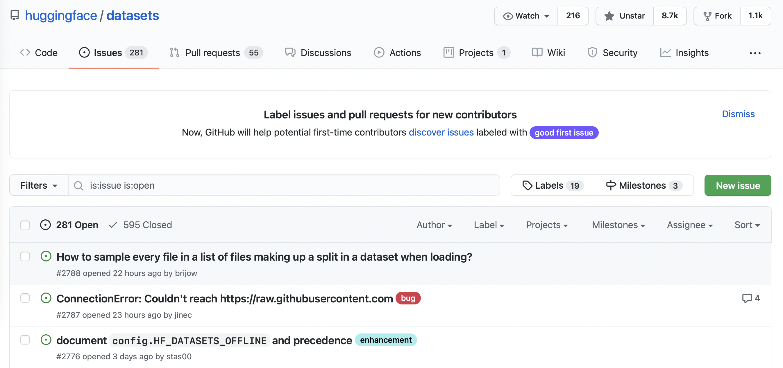
If you click on one of these issues you’ll find it contains a title, a description, and a set of labels that characterize the issue. An example is shown in the screenshot below.
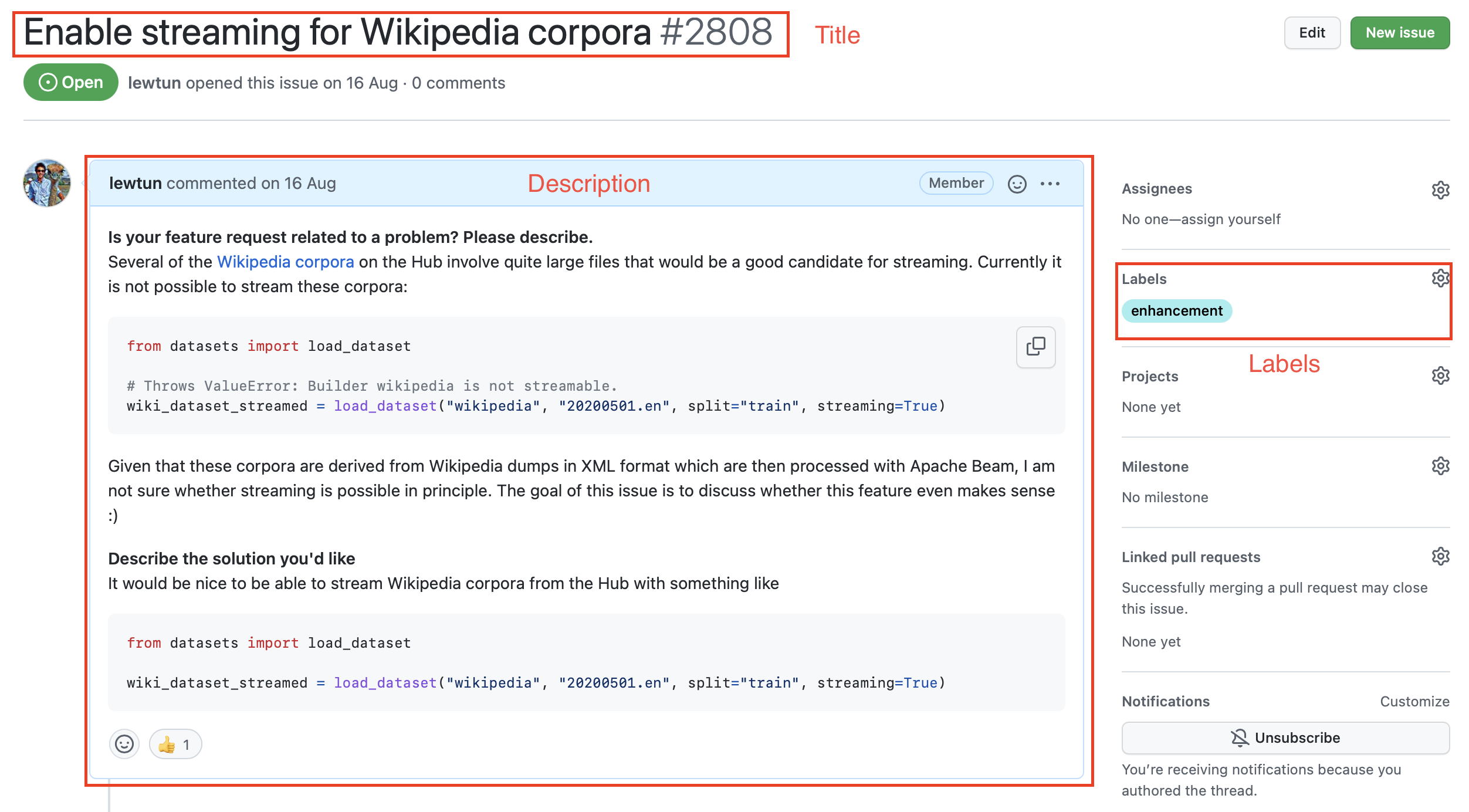
To download all the repository’s issues, we’ll use the GitHub REST API to poll the Issues endpoint. This endpoint returns a list of JSON objects, with each object containing a large number of fields that include the title and description as well as metadata about the status of the issue and so on.
A convenient way to download the issues is via the requests library, which is the standard way for making HTTP requests in Python. You can install the library by running:
!pip install requests
Once the library is installed, you can make GET requests to the Issues endpoint by invoking the requests.get() function. For example, you can run the following command to retrieve the first issue on the first page:
import requests
url = "https://api.github.com/repos/huggingface/datasets/issues?page=1&per_page=1"
response = requests.get(url)
The response object contains a lot of useful information about the request, including the HTTP status code:
response.status_code
200
where a 200 status means the request was successful (you can find a list of possible HTTP status codes here). What we are really interested in, though, is the payload, which can be accessed in various formats like bytes, strings, or JSON. Since we know our issues are in JSON format, let’s inspect the payload as follows:
response.json()
[{'url': 'https://api.github.com/repos/huggingface/datasets/issues/2792',
'repository_url': 'https://api.github.com/repos/huggingface/datasets',
'labels_url': 'https://api.github.com/repos/huggingface/datasets/issues/2792/labels{/name}',
'comments_url': 'https://api.github.com/repos/huggingface/datasets/issues/2792/comments',
'events_url': 'https://api.github.com/repos/huggingface/datasets/issues/2792/events',
'html_url': 'https://github.com/huggingface/datasets/pull/2792',
'id': 968650274,
'node_id': 'MDExOlB1bGxSZXF1ZXN0NzEwNzUyMjc0',
'number': 2792,
'title': 'Update GooAQ',
'user': {'login': 'bhavitvyamalik',
'id': 19718818,
'node_id': 'MDQ6VXNlcjE5NzE4ODE4',
'avatar_url': 'https://avatars.githubusercontent.com/u/19718818?v=4',
'gravatar_id': '',
'url': 'https://api.github.com/users/bhavitvyamalik',
'html_url': 'https://github.com/bhavitvyamalik',
'followers_url': 'https://api.github.com/users/bhavitvyamalik/followers',
'following_url': 'https://api.github.com/users/bhavitvyamalik/following{/other_user}',
'gists_url': 'https://api.github.com/users/bhavitvyamalik/gists{/gist_id}',
'starred_url': 'https://api.github.com/users/bhavitvyamalik/starred{/owner}{/repo}',
'subscriptions_url': 'https://api.github.com/users/bhavitvyamalik/subscriptions',
'organizations_url': 'https://api.github.com/users/bhavitvyamalik/orgs',
'repos_url': 'https://api.github.com/users/bhavitvyamalik/repos',
'events_url': 'https://api.github.com/users/bhavitvyamalik/events{/privacy}',
'received_events_url': 'https://api.github.com/users/bhavitvyamalik/received_events',
'type': 'User',
'site_admin': False},
'labels': [],
'state': 'open',
'locked': False,
'assignee': None,
'assignees': [],
'milestone': None,
'comments': 1,
'created_at': '2021-08-12T11:40:18Z',
'updated_at': '2021-08-12T12:31:17Z',
'closed_at': None,
'author_association': 'CONTRIBUTOR',
'active_lock_reason': None,
'pull_request': {'url': 'https://api.github.com/repos/huggingface/datasets/pulls/2792',
'html_url': 'https://github.com/huggingface/datasets/pull/2792',
'diff_url': 'https://github.com/huggingface/datasets/pull/2792.diff',
'patch_url': 'https://github.com/huggingface/datasets/pull/2792.patch'},
'body': '[GooAQ](https://github.com/allenai/gooaq) dataset was recently updated after splits were added for the same. This PR contains new updated GooAQ with train/val/test splits and updated README as well.',
'performed_via_github_app': None}]
Whoa, that’s a lot of information! We can see useful fields like title, body, and number that describe the issue, as well as information about the GitHub user who opened the issue.
[!TIP] ✏️ Try it out! Click on a few of the URLs in the JSON payload above to get a feel for what type of information each GitHub issue is linked to.
As described in the GitHub documentation, unauthenticated requests are limited to 60 requests per hour. Although you can increase the per_page query parameter to reduce the number of requests you make, you will still hit the rate limit on any repository that has more than a few thousand issues. So instead, you should follow GitHub’s instructions on creating a personal access token so that you can boost the rate limit to 5,000 requests per hour. Once you have your token, you can include it as part of the request header:
GITHUB_TOKEN = xxx ### Copy your GitHub token here
headers = {"Authorization": f"token {GITHUB_TOKEN}"}
[!WARNING] ⚠️ Do not share a notebook with your
GITHUB_TOKENpasted in it. We recommend you delete the last cell once you have executed it to avoid leaking this information accidentally. Even better, store the token in a .env file and use thepython-dotenvlibrary to load it automatically for you as an environment variable.
Now that we have our access token, let’s create a function that can download all the issues from a GitHub repository:
import time
import math
from pathlib import Path
import pandas as pd
from tqdm.notebook import tqdm
def fetch_issues(
owner="huggingface",
repo="datasets",
num_issues=10_000,
rate_limit=5_000,
issues_path=Path("."),
):
if not issues_path.is_dir():
issues_path.mkdir(exist_ok=True)
batch = []
all_issues = []
per_page = 100 ### Number of issues to return per page
num_pages = math.ceil(num_issues / per_page)
base_url = "https://api.github.com/repos"
for page in tqdm(range(num_pages)):
### Query with state=all to get both open and closed issues
query = f"issues?page={page}&per_page={per_page}&state=all"
issues = requests.get(f"{base_url}/{owner}/{repo}/{query}", headers=headers)
batch.extend(issues.json())
if len(batch) > rate_limit and len(all_issues) < num_issues:
all_issues.extend(batch)
batch = [] ### Flush batch for next time period
print(f"Reached GitHub rate limit. Sleeping for one hour ...")
time.sleep(60 * 60 + 1)
all_issues.extend(batch)
df = pd.DataFrame.from_records(all_issues)
df.to_json(f"{issues_path}/{repo}-issues.jsonl", orient="records", lines=True)
print(
f"Downloaded all the issues for {repo}! Dataset stored at {issues_path}/{repo}-issues.jsonl"
)
Now when we call fetch_issues() it will download all the issues in batches to avoid exceeding GitHub’s limit on the number of requests per hour; the result will be stored in a repository_name-issues.jsonl file, where each line is a JSON object the represents an issue. Let’s use this function to grab all the issues from 🤗 Datasets:
### Depending on your internet connection, this can take several minutes to run...
fetch_issues()
Once the issues are downloaded we can load them locally using our newfound skills from section 2:
issues_dataset = load_dataset("json", data_files="datasets-issues.jsonl", split="train")
issues_dataset
Dataset({
features: ['url', 'repository_url', 'labels_url', 'comments_url', 'events_url', 'html_url', 'id', 'node_id', 'number', 'title', 'user', 'labels', 'state', 'locked', 'assignee', 'assignees', 'milestone', 'comments', 'created_at', 'updated_at', 'closed_at', 'author_association', 'active_lock_reason', 'pull_request', 'body', 'timeline_url', 'performed_via_github_app'],
num_rows: 3019
})
Great, we’ve created our first dataset from scratch! But why are there several thousand issues when the Issues tab of the 🤗 Datasets repository only shows around 1,000 issues in total 🤔? As described in the GitHub documentation, that’s because we’ve downloaded all the pull requests as well:
GitHub’s REST API v3 considers every pull request an issue, but not every issue is a pull request. For this reason, “Issues” endpoints may return both issues and pull requests in the response. You can identify pull requests by the
pull_requestkey. Be aware that theidof a pull request returned from “Issues” endpoints will be an issue id.
Since the contents of issues and pull requests are quite different, let’s do some minor preprocessing to enable us to distinguish between them.
Cleaning up the data
The above snippet from GitHub’s documentation tells us that the pull_request column can be used to differentiate between issues and pull requests. Let’s look at a random sample to see what the difference is. As we did in section 3, we’ll chain Dataset.shuffle() and Dataset.select() to create a random sample and then zip the html_url and pull_request columns so we can compare the various URLs:
sample = issues_dataset.shuffle(seed=666).select(range(3))
### Print out the URL and pull request entries
for url, pr in zip(sample["html_url"], sample["pull_request"]):
print(f">> URL: {url}")
print(f">> Pull request: {pr}\n")
>> URL: https://github.com/huggingface/datasets/pull/850
>> Pull request: {'url': 'https://api.github.com/repos/huggingface/datasets/pulls/850', 'html_url': 'https://github.com/huggingface/datasets/pull/850', 'diff_url': 'https://github.com/huggingface/datasets/pull/850.diff', 'patch_url': 'https://github.com/huggingface/datasets/pull/850.patch'}
>> URL: https://github.com/huggingface/datasets/issues/2773
>> Pull request: None
>> URL: https://github.com/huggingface/datasets/pull/783
>> Pull request: {'url': 'https://api.github.com/repos/huggingface/datasets/pulls/783', 'html_url': 'https://github.com/huggingface/datasets/pull/783', 'diff_url': 'https://github.com/huggingface/datasets/pull/783.diff', 'patch_url': 'https://github.com/huggingface/datasets/pull/783.patch'}
Here we can see that each pull request is associated with various URLs, while ordinary issues have a None entry. We can use this distinction to create a new is_pull_request column that checks whether the pull_request field is None or not:
issues_dataset = issues_dataset.map(
lambda x: {"is_pull_request": False if x["pull_request"] is None else True}
)
[!TIP] ✏️ Try it out! Calculate the average time it takes to close issues in 🤗 Datasets. You may find the
Dataset.filter()function useful to filter out the pull requests and open issues, and you can use theDataset.set_format()function to convert the dataset to aDataFrameso you can easily manipulate thecreated_atandclosed_attimestamps. For bonus points, calculate the average time it takes to close pull requests.
Although we could proceed to further clean up the dataset by dropping or renaming some columns, it is generally a good practice to keep the dataset as “raw” as possible at this stage so that it can be easily used in multiple applications.
Before we push our dataset to the Hugging Face Hub, let’s deal with one thing that’s missing from it: the comments associated with each issue and pull request. We’ll add them next with – you guessed it – the GitHub REST API!
Augmenting the dataset
As shown in the following screenshot, the comments associated with an issue or pull request provide a rich source of information, especially if we’re interested in building a search engine to answer user queries about the library.
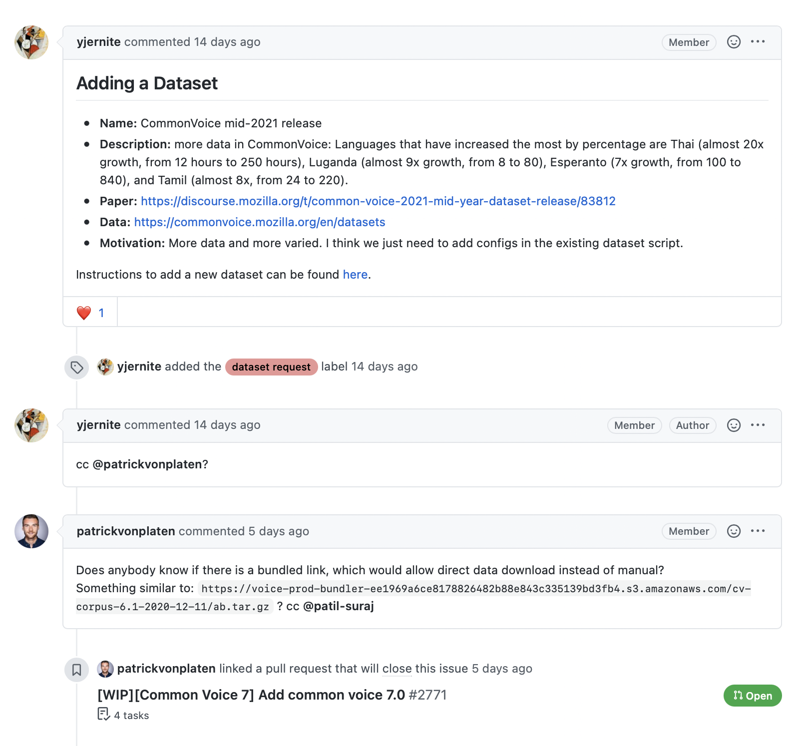
The GitHub REST API provides a Comments endpoint that returns all the comments associated with an issue number. Let’s test the endpoint to see what it returns:
issue_number = 2792
url = f"https://api.github.com/repos/huggingface/datasets/issues/{issue_number}/comments"
response = requests.get(url, headers=headers)
response.json()
[{'url': 'https://api.github.com/repos/huggingface/datasets/issues/comments/897594128',
'html_url': 'https://github.com/huggingface/datasets/pull/2792#issuecomment-897594128',
'issue_url': 'https://api.github.com/repos/huggingface/datasets/issues/2792',
'id': 897594128,
'node_id': 'IC_kwDODunzps41gDMQ',
'user': {'login': 'bhavitvyamalik',
'id': 19718818,
'node_id': 'MDQ6VXNlcjE5NzE4ODE4',
'avatar_url': 'https://avatars.githubusercontent.com/u/19718818?v=4',
'gravatar_id': '',
'url': 'https://api.github.com/users/bhavitvyamalik',
'html_url': 'https://github.com/bhavitvyamalik',
'followers_url': 'https://api.github.com/users/bhavitvyamalik/followers',
'following_url': 'https://api.github.com/users/bhavitvyamalik/following{/other_user}',
'gists_url': 'https://api.github.com/users/bhavitvyamalik/gists{/gist_id}',
'starred_url': 'https://api.github.com/users/bhavitvyamalik/starred{/owner}{/repo}',
'subscriptions_url': 'https://api.github.com/users/bhavitvyamalik/subscriptions',
'organizations_url': 'https://api.github.com/users/bhavitvyamalik/orgs',
'repos_url': 'https://api.github.com/users/bhavitvyamalik/repos',
'events_url': 'https://api.github.com/users/bhavitvyamalik/events{/privacy}',
'received_events_url': 'https://api.github.com/users/bhavitvyamalik/received_events',
'type': 'User',
'site_admin': False},
'created_at': '2021-08-12T12:21:52Z',
'updated_at': '2021-08-12T12:31:17Z',
'author_association': 'CONTRIBUTOR',
'body': "@albertvillanova my tests are failing here:\r\n```\r\ndataset_name = 'gooaq'\r\n\r\n def test_load_dataset(self, dataset_name):\r\n configs = self.dataset_tester.load_all_configs(dataset_name, is_local=True)[:1]\r\n> self.dataset_tester.check_load_dataset(dataset_name, configs, is_local=True, use_local_dummy_data=True)\r\n\r\ntests/test_dataset_common.py:234: \r\n_ _ _ _ _ _ _ _ _ _ _ _ _ _ _ _ _ _ _ _ _ _ _ _ _ _ _ _ _ _ _ _ _ _ _ _ _ _ _ _ \r\ntests/test_dataset_common.py:187: in check_load_dataset\r\n self.parent.assertTrue(len(dataset[split]) > 0)\r\nE AssertionError: False is not true\r\n```\r\nWhen I try loading dataset on local machine it works fine. Any suggestions on how can I avoid this error?",
'performed_via_github_app': None}]
We can see that the comment is stored in the body field, so let’s write a simple function that returns all the comments associated with an issue by picking out the body contents for each element in response.json():
def get_comments(issue_number):
url = f"https://api.github.com/repos/huggingface/datasets/issues/{issue_number}/comments"
response = requests.get(url, headers=headers)
return [r["body"] for r in response.json()]
### Test our function works as expected
get_comments(2792)
["@albertvillanova my tests are failing here:\r\n```\r\ndataset_name = 'gooaq'\r\n\r\n def test_load_dataset(self, dataset_name):\r\n configs = self.dataset_tester.load_all_configs(dataset_name, is_local=True)[:1]\r\n> self.dataset_tester.check_load_dataset(dataset_name, configs, is_local=True, use_local_dummy_data=True)\r\n\r\ntests/test_dataset_common.py:234: \r\n_ _ _ _ _ _ _ _ _ _ _ _ _ _ _ _ _ _ _ _ _ _ _ _ _ _ _ _ _ _ _ _ _ _ _ _ _ _ _ _ \r\ntests/test_dataset_common.py:187: in check_load_dataset\r\n self.parent.assertTrue(len(dataset[split]) > 0)\r\nE AssertionError: False is not true\r\n```\r\nWhen I try loading dataset on local machine it works fine. Any suggestions on how can I avoid this error?"]
This looks good, so let’s use Dataset.map() to add a new comments column to each issue in our dataset:
### Depending on your internet connection, this can take a few minutes...
issues_with_comments_dataset = issues_dataset.map(
lambda x: {"comments": get_comments(x["number"])}
)
The final step is to push our dataset to the Hub. Let’s take a look at how we can do that.
Uploading the dataset to the Hugging Face Hub
Now that we have our augmented dataset, it’s time to push it to the Hub so we can share it with the community! Uploading a dataset is very simple: just like models and tokenizers from 🤗 Transformers, we can use a push_to_hub() method to push a dataset. To do that we need an authentication token, which can be obtained by first logging into the Hugging Face Hub with the notebook_login() function:
from huggingface_hub import notebook_login
notebook_login()
This will create a widget where you can enter your username and password, and an API token will be saved in ~/.huggingface/token. If you’re running the code in a terminal, you can log in via the CLI instead:
huggingface-cli login
Once we’ve done this, we can upload our dataset by running:
issues_with_comments_dataset.push_to_hub("github-issues")
From here, anyone can download the dataset by simply providing load_dataset() with the repository ID as the path argument:
remote_dataset = load_dataset("lewtun/github-issues", split="train")
remote_dataset
Dataset({
features: ['url', 'repository_url', 'labels_url', 'comments_url', 'events_url', 'html_url', 'id', 'node_id', 'number', 'title', 'user', 'labels', 'state', 'locked', 'assignee', 'assignees', 'milestone', 'comments', 'created_at', 'updated_at', 'closed_at', 'author_association', 'active_lock_reason', 'pull_request', 'body', 'performed_via_github_app', 'is_pull_request'],
num_rows: 2855
})
Cool, we’ve pushed our dataset to the Hub and it’s available for others to use! There’s just one important thing left to do: adding a dataset card that explains how the corpus was created and provides other useful information for the community.
[!TIP] 💡 You can also upload a dataset to the Hugging Face Hub directly from the terminal by using
huggingface-cliand a bit of Git magic. See the 🤗 Datasets guide for details on how to do this.
Creating a dataset card
Well-documented datasets are more likely to be useful to others (including your future self!), as they provide the context to enable users to decide whether the dataset is relevant to their task and to evaluate any potential biases in or risks associated with using the dataset.
On the Hugging Face Hub, this information is stored in each dataset repository’s README.md file. There are two main steps you should take before creating this file:
- Use the
datasets-taggingapplication to create metadata tags in YAML format. These tags are used for a variety of search features on the Hugging Face Hub and ensure your dataset can be easily found by members of the community. Since we have created a custom dataset here, you’ll need to clone thedatasets-taggingrepository and run the application locally. Here’s what the interface looks like:

- Read the 🤗 Datasets guide on creating informative dataset cards and use it as a template.
You can create the README.md file directly on the Hub, and you can find a template dataset card in the lewtun/github-issues dataset repository. A screenshot of the filled-out dataset card is shown below.
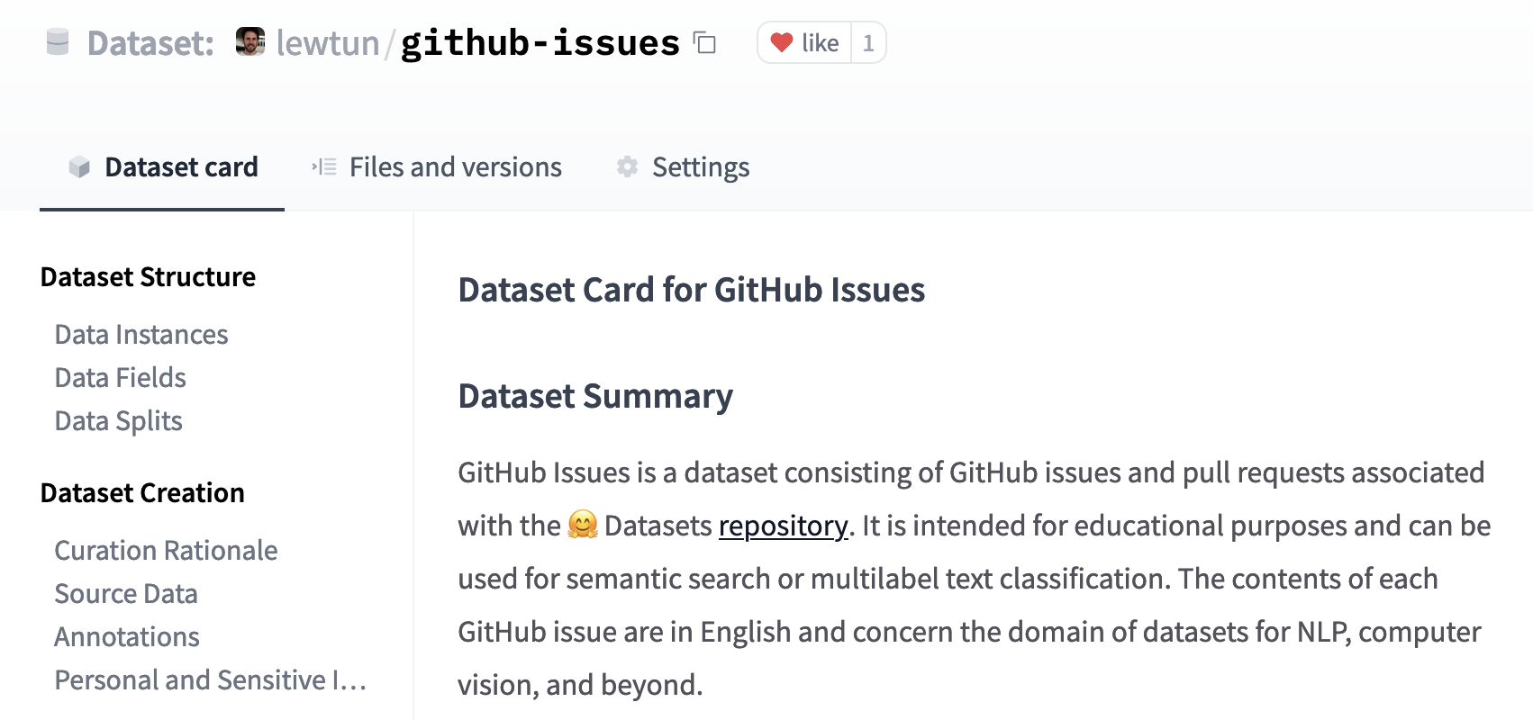
[!TIP] ✏️ Try it out! Use the
dataset-taggingapplication and 🤗 Datasets guide to complete the README.md file for your GitHub issues dataset.
That’s it! We’ve seen in this section that creating a good dataset can be quite involved, but fortunately uploading it and sharing it with the community is not. In the next section we’ll use our new dataset to create a semantic search engine with 🤗 Datasets that can match questions to the most relevant issues and comments.
[!TIP] ✏️ Try it out! Go through the steps we took in this section to create a dataset of GitHub issues for your favorite open source library (pick something other than 🤗 Datasets, of course!). For bonus points, fine-tune a multilabel classifier to predict the tags present in the
labelsfield.
6. Semantic search with FAISS
In section 5, we created a dataset of GitHub issues and comments from the 🤗 Datasets repository. In this section we’ll use this information to build a search engine that can help us find answers to our most pressing questions about the library!
Using embeddings for semantic search
As we saw in Chapter 1, Transformer-based language models represent each token in a span of text as an embedding vector. It turns out that one can “pool” the individual embeddings to create a vector representation for whole sentences, paragraphs, or (in some cases) documents. These embeddings can then be used to find similar documents in the corpus by computing the dot-product similarity (or some other similarity metric) between each embedding and returning the documents with the greatest overlap.
In this section we’ll use embeddings to develop a semantic search engine. These search engines offer several advantages over conventional approaches that are based on matching keywords in a query with the documents.


Loading and preparing the dataset
The first thing we need to do is download our dataset of GitHub issues, so let’s use load_dataset() function as usual:
from datasets import load_dataset
issues_dataset = load_dataset("lewtun/github-issues", split="train")
issues_dataset
Dataset({
features: ['url', 'repository_url', 'labels_url', 'comments_url', 'events_url', 'html_url', 'id', 'node_id', 'number', 'title', 'user', 'labels', 'state', 'locked', 'assignee', 'assignees', 'milestone', 'comments', 'created_at', 'updated_at', 'closed_at', 'author_association', 'active_lock_reason', 'pull_request', 'body', 'performed_via_github_app', 'is_pull_request'],
num_rows: 2855
})
Here we’ve specified the default train split in load_dataset(), so it returns a Dataset instead of a DatasetDict. The first order of business is to filter out the pull requests, as these tend to be rarely used for answering user queries and will introduce noise in our search engine. As should be familiar by now, we can use the Dataset.filter() function to exclude these rows in our dataset. While we’re at it, let’s also filter out rows with no comments, since these provide no answers to user queries:
issues_dataset = issues_dataset.filter(
lambda x: (x["is_pull_request"] == False and len(x["comments"]) > 0)
)
issues_dataset
Dataset({
features: ['url', 'repository_url', 'labels_url', 'comments_url', 'events_url', 'html_url', 'id', 'node_id', 'number', 'title', 'user', 'labels', 'state', 'locked', 'assignee', 'assignees', 'milestone', 'comments', 'created_at', 'updated_at', 'closed_at', 'author_association', 'active_lock_reason', 'pull_request', 'body', 'performed_via_github_app', 'is_pull_request'],
num_rows: 771
})
We can see that there are a lot of columns in our dataset, most of which we don’t need to build our search engine. From a search perspective, the most informative columns are title, body, and comments, while html_url provides us with a link back to the source issue. Let’s use the Dataset.remove_columns() function to drop the rest:
columns = issues_dataset.column_names
columns_to_keep = ["title", "body", "html_url", "comments"]
columns_to_remove = set(columns_to_keep).symmetric_difference(columns)
issues_dataset = issues_dataset.remove_columns(columns_to_remove)
issues_dataset
Dataset({
features: ['html_url', 'title', 'comments', 'body'],
num_rows: 771
})
To create our embeddings we’ll augment each comment with the issue’s title and body, since these fields often include useful contextual information. Because our comments column is currently a list of comments for each issue, we need to “explode” the column so that each row consists of an (html_url, title, body, comment) tuple. In Pandas we can do this with the DataFrame.explode() function, which creates a new row for each element in a list-like column, while replicating all the other column values. To see this in action, let’s first switch to the Pandas DataFrame format:
issues_dataset.set_format("pandas")
df = issues_dataset[:]
If we inspect the first row in this DataFrame we can see there are four comments associated with this issue:
df["comments"][0].tolist()
['the bug code locate in :\r\n if data_args.task_name is not None:\r\n ### Downloading and loading a dataset from the hub.\r\n datasets = load_dataset("glue", data_args.task_name, cache_dir=model_args.cache_dir)',
'Hi @jinec,\r\n\r\nFrom time to time we get this kind of `ConnectionError` coming from the github.com website: https://raw.githubusercontent.com\r\n\r\nNormally, it should work if you wait a little and then retry.\r\n\r\nCould you please confirm if the problem persists?',
'cannot connect,even by Web browser,please check that there is some problems。',
'I can access https://raw.githubusercontent.com/huggingface/datasets/1.7.0/datasets/glue/glue.py without problem...']
When we explode df, we expect to get one row for each of these comments. Let’s check if that’s the case:
comments_df = df.explode("comments", ignore_index=True)
comments_df.head(4)
| html_url | title | comments | body | |
|---|---|---|---|---|
| 0 | https://github.com/huggingface/datasets/issues/2787 | ConnectionError: Couldn't reach https://raw.githubusercontent.com | the bug code locate in :\r\n if data_args.task_name is not None... | Hello,\r\nI am trying to run run_glue.py and it gives me this error... |
| 1 | https://github.com/huggingface/datasets/issues/2787 | ConnectionError: Couldn't reach https://raw.githubusercontent.com | Hi @jinec,\r\n\r\nFrom time to time we get this kind of `ConnectionError` coming from the github.com website: https://raw.githubusercontent.com... | Hello,\r\nI am trying to run run_glue.py and it gives me this error... |
| 2 | https://github.com/huggingface/datasets/issues/2787 | ConnectionError: Couldn't reach https://raw.githubusercontent.com | cannot connect,even by Web browser,please check that there is some problems。 | Hello,\r\nI am trying to run run_glue.py and it gives me this error... |
| 3 | https://github.com/huggingface/datasets/issues/2787 | ConnectionError: Couldn't reach https://raw.githubusercontent.com | I can access https://raw.githubusercontent.com/huggingface/datasets/1.7.0/datasets/glue/glue.py without problem... | Hello,\r\nI am trying to run run_glue.py and it gives me this error... |
Great, we can see the rows have been replicated, with the comments column containing the individual comments! Now that we’re finished with Pandas, we can quickly switch back to a Dataset by loading the DataFrame in memory:
from datasets import Dataset
comments_dataset = Dataset.from_pandas(comments_df)
comments_dataset
Dataset({
features: ['html_url', 'title', 'comments', 'body'],
num_rows: 2842
})
Okay, this has given us a few thousand comments to work with!
[!TIP] ✏️ Try it out! See if you can use
Dataset.map()to explode thecommentscolumn ofissues_datasetwithout resorting to the use of Pandas. This is a little tricky; you might find the “Batch mapping” section of the 🤗 Datasets documentation useful for this task.
Now that we have one comment per row, let’s create a new comments_length column that contains the number of words per comment:
comments_dataset = comments_dataset.map(
lambda x: {"comment_length": len(x["comments"].split())}
)
We can use this new column to filter out short comments, which typically include things like “cc @lewtun” or “Thanks!” that are not relevant for our search engine. There’s no precise number to select for the filter, but around 15 words seems like a good start:
comments_dataset = comments_dataset.filter(lambda x: x["comment_length"] > 15)
comments_dataset
Dataset({
features: ['html_url', 'title', 'comments', 'body', 'comment_length'],
num_rows: 2098
})
Having cleaned up our dataset a bit, let’s concatenate the issue title, description, and comments together in a new text column. As usual, we’ll write a simple function that we can pass to Dataset.map():
def concatenate_text(examples):
return {
"text": examples["title"]
+ " \n "
+ examples["body"]
+ " \n "
+ examples["comments"]
}
comments_dataset = comments_dataset.map(concatenate_text)
We’re finally ready to create some embeddings! Let’s take a look.
Creating text embeddings
We saw in Chapter 2 that we can obtain token embeddings by using the AutoModel class. All we need to do is pick a suitable checkpoint to load the model from. Fortunately, there’s a library called sentence-transformers that is dedicated to creating embeddings. As described in the library’s documentation, our use case is an example of asymmetric semantic search because we have a short query whose answer we’d like to find in a longer document, like a an issue comment. The handy model overview table in the documentation indicates that the multi-qa-mpnet-base-dot-v1 checkpoint has the best performance for semantic search, so we’ll use that for our application. We’ll also load the tokenizer using the same checkpoint:
from transformers import AutoTokenizer, AutoModel
model_ckpt = "sentence-transformers/multi-qa-mpnet-base-dot-v1"
tokenizer = AutoTokenizer.from_pretrained(model_ckpt)
model = AutoModel.from_pretrained(model_ckpt)
To speed up the embedding process, it helps to place the model and inputs on a GPU device, so let’s do that now:
import torch
device = torch.device("cuda")
model.to(device)
As we mentioned earlier, we’d like to represent each entry in our GitHub issues corpus as a single vector, so we need to “pool” or average our token embeddings in some way. One popular approach is to perform CLS pooling on our model’s outputs, where we simply collect the last hidden state for the special [CLS] token. The following function does the trick for us:
def cls_pooling(model_output):
return model_output.last_hidden_state[:, 0]
Next, we’ll create a helper function that will tokenize a list of documents, place the tensors on the GPU, feed them to the model, and finally apply CLS pooling to the outputs:
def get_embeddings(text_list):
encoded_input = tokenizer(
text_list, padding=True, truncation=True, return_tensors="pt"
)
encoded_input = {k: v.to(device) for k, v in encoded_input.items()}
model_output = model(**encoded_input)
return cls_pooling(model_output)
We can test the function works by feeding it the first text entry in our corpus and inspecting the output shape:
embedding = get_embeddings(comments_dataset["text"][0])
embedding.shape
torch.Size([1, 768])
Great, we’ve converted the first entry in our corpus into a 768-dimensional vector! We can use Dataset.map() to apply our get_embeddings() function to each row in our corpus, so let’s create a new embeddings column as follows:
embeddings_dataset = comments_dataset.map(
lambda x: {"embeddings": get_embeddings(x["text"]).detach().cpu().numpy()[0]}
)
Notice that we’ve converted the embeddings to NumPy arrays – that’s because 🤗 Datasets requires this format when we try to index them with FAISS, which we’ll do next.
Using FAISS for efficient similarity search
Now that we have a dataset of embeddings, we need some way to search over them. To do this, we’ll use a special data structure in 🤗 Datasets called a FAISS index. FAISS (short for Facebook AI Similarity Search) is a library that provides efficient algorithms to quickly search and cluster embedding vectors.
The basic idea behind FAISS is to create a special data structure called an index that allows one to find which embeddings are similar to an input embedding. Creating a FAISS index in 🤗 Datasets is simple – we use the Dataset.add_faiss_index() function and specify which column of our dataset we’d like to index:
embeddings_dataset.add_faiss_index(column="embeddings")
We can now perform queries on this index by doing a nearest neighbor lookup with the Dataset.get_nearest_examples() function. Let’s test this out by first embedding a question as follows:
{#if fw === ‘pt’}
question = "How can I load a dataset offline?"
question_embedding = get_embeddings([question]).cpu().detach().numpy()
question_embedding.shape
torch.Size([1, 768])
question = "How can I load a dataset offline?"
question_embedding = get_embeddings([question]).numpy()
question_embedding.shape
(1, 768)
{/if}
Just like with the documents, we now have a 768-dimensional vector representing the query, which we can compare against the whole corpus to find the most similar embeddings:
scores, samples = embeddings_dataset.get_nearest_examples(
"embeddings", question_embedding, k=5
)
The Dataset.get_nearest_examples() function returns a tuple of scores that rank the overlap between the query and the document, and a corresponding set of samples (here, the 5 best matches). Let’s collect these in a pandas.DataFrame so we can easily sort them:
import pandas as pd
samples_df = pd.DataFrame.from_dict(samples)
samples_df["scores"] = scores
samples_df.sort_values("scores", ascending=False, inplace=True)
Now we can iterate over the first few rows to see how well our query matched the available comments:
for _, row in samples_df.iterrows():
print(f"COMMENT: {row.comments}")
print(f"SCORE: {row.scores}")
print(f"TITLE: {row.title}")
print(f"URL: {row.html_url}")
print("=" * 50)
print()
"""
COMMENT: Requiring online connection is a deal breaker in some cases unfortunately so it'd be great if offline mode is added similar to how `transformers` loads models offline fine.
@mandubian's second bullet point suggests that there's a workaround allowing you to use your offline (custom?) dataset with `datasets`. Could you please elaborate on how that should look like?
SCORE: 25.505046844482422
TITLE: Discussion using datasets in offline mode
URL: https://github.com/huggingface/datasets/issues/824
==================================================
COMMENT: The local dataset builders (csv, text , json and pandas) are now part of the `datasets` package since #1726 :)
You can now use them offline
\`\`\`python
datasets = load_dataset("text", data_files=data_files)
\`\`\`
We'll do a new release soon
SCORE: 24.555509567260742
TITLE: Discussion using datasets in offline mode
URL: https://github.com/huggingface/datasets/issues/824
==================================================
COMMENT: I opened a PR that allows to reload modules that have already been loaded once even if there's no internet.
Let me know if you know other ways that can make the offline mode experience better. I'd be happy to add them :)
I already note the "freeze" modules option, to prevent local modules updates. It would be a cool feature.
----------
> @mandubian's second bullet point suggests that there's a workaround allowing you to use your offline (custom?) dataset with `datasets`. Could you please elaborate on how that should look like?
Indeed `load_dataset` allows to load remote dataset script (squad, glue, etc.) but also you own local ones.
For example if you have a dataset script at `./my_dataset/my_dataset.py` then you can do
\`\`\`python
load_dataset("./my_dataset")
\`\`\`
and the dataset script will generate your dataset once and for all.
----------
About I'm looking into having `csv`, `json`, `text`, `pandas` dataset builders already included in the `datasets` package, so that they are available offline by default, as opposed to the other datasets that require the script to be downloaded.
cf #1724
SCORE: 24.14896583557129
TITLE: Discussion using datasets in offline mode
URL: https://github.com/huggingface/datasets/issues/824
==================================================
COMMENT: > here is my way to load a dataset offline, but it **requires** an online machine
>
> 1. (online machine)
>
> ```
>
> import datasets
>
> data = datasets.load_dataset(...)
>
> data.save_to_disk(/YOUR/DATASET/DIR)
>
> ```
>
> 2. copy the dir from online to the offline machine
>
> 3. (offline machine)
>
> ```
>
> import datasets
>
> data = datasets.load_from_disk(/SAVED/DATA/DIR)
>
> ```
>
>
>
> HTH.
SCORE: 22.893993377685547
TITLE: Discussion using datasets in offline mode
URL: https://github.com/huggingface/datasets/issues/824
==================================================
COMMENT: here is my way to load a dataset offline, but it **requires** an online machine
1. (online machine)
\`\`\`
import datasets
data = datasets.load_dataset(...)
data.save_to_disk(/YOUR/DATASET/DIR)
\`\`\`
2. copy the dir from online to the offline machine
3. (offline machine)
\`\`\`
import datasets
data = datasets.load_from_disk(/SAVED/DATA/DIR)
\`\`\`
HTH.
SCORE: 22.406635284423828
TITLE: Discussion using datasets in offline mode
URL: https://github.com/huggingface/datasets/issues/824
==================================================
"""
Not bad! Our second hit seems to match the query.
[!TIP] ✏️ Try it out! Create your own query and see whether you can find an answer in the retrieved documents. You might have to increase the
kparameter inDataset.get_nearest_examples()to broaden the search.
7. 🤗 Datasets, check!
Well, that was quite a tour through the 🤗 Datasets library – congratulations on making it this far! With the knowledge that you’ve gained from this chapter, you should be able to:
- Load datasets from anywhere, be it the Hugging Face Hub, your laptop, or a remote server at your company.
- Wrangle your data using a mix of the
Dataset.map()andDataset.filter()functions. - Quickly switch between data formats like Pandas and NumPy using
Dataset.set_format(). - Create your very own dataset and push it to the Hugging Face Hub.
- Embed your documents using a Transformer model and build a semantic search engine using FAISS.
In Chapter 7, we’ll put all of this to good use as we take a deep dive into the core NLP tasks that Transformer models are great for. Before jumping ahead, though, put your knowledge of 🤗 Datasets to the test with a quick quiz!
Chapter 6. The 🤗 Tokenizers library
1. Introduction
In Chapter 3, we looked at how to fine-tune a model on a given task. When we do that, we use the same tokenizer that the model was pretrained with – but what do we do when we want to train a model from scratch? In these cases, using a tokenizer that was pretrained on a corpus from another domain or language is typically suboptimal. For example, a tokenizer that’s trained on an English corpus will perform poorly on a corpus of Japanese texts because the use of spaces and punctuation is very different in the two languages.
In this chapter, you will learn how to train a brand new tokenizer on a corpus of texts, so it can then be used to pretrain a language model. This will all be done with the help of the 🤗 Tokenizers library, which provides the “fast” tokenizers in the 🤗 Transformers library. We’ll take a close look at the features that this library provides, and explore how the fast tokenizers differ from the “slow” versions.
Topics we will cover include:
- How to train a new tokenizer similar to the one used by a given checkpoint on a new corpus of texts
- The special features of fast tokenizers
- The differences between the three main subword tokenization algorithms used in NLP today
- How to build a tokenizer from scratch with the 🤗 Tokenizers library and train it on some data
The techniques introduced in this chapter will prepare you for the section in Chapter 7 where we look at creating a language model for Python source code. Let’s start by looking at what it means to “train” a tokenizer in the first place.
2. Training a new tokenizer from an old one
If a language model is not available in the language you are interested in, or if your corpus is very different from the one your language model was trained on, you will most likely want to retrain the model from scratch using a tokenizer adapted to your data. That will require training a new tokenizer on your dataset. But what exactly does that mean? When we first looked at tokenizers in Chapter 2, we saw that most Transformer models use a subword tokenization algorithm. To identify which subwords are of interest and occur most frequently in the corpus at hand, the tokenizer needs to take a hard look at all the texts in the corpus – a process we call training. The exact rules that govern this training depend on the type of tokenizer used, and we’ll go over the three main algorithms later in this chapter.
[!WARNING] ⚠️ Training a tokenizer is not the same as training a model! Model training uses stochastic gradient descent to make the loss a little bit smaller for each batch. It’s randomized by nature (meaning you have to set some seeds to get the same results when doing the same training twice). Training a tokenizer is a statistical process that tries to identify which subwords are the best to pick for a given corpus, and the exact rules used to pick them depend on the tokenization algorithm. It’s deterministic, meaning you always get the same results when training with the same algorithm on the same corpus.
Assembling a corpus
There’s a very simple API in 🤗 Transformers that you can use to train a new tokenizer with the same characteristics as an existing one: AutoTokenizer.train_new_from_iterator(). To see this in action, let’s say we want to train GPT-2 from scratch, but in a language other than English. Our first task will be to gather lots of data in that language in a training corpus. To provide examples everyone will be able to understand, we won’t use a language like Russian or Chinese here, but rather a specialized English language: Python code.
The 🤗 Datasets library can help us assemble a corpus of Python source code. We’ll use the usual load_dataset() function to download and cache the CodeSearchNet dataset. This dataset was created for the CodeSearchNet challenge and contains millions of functions from open source libraries on GitHub in several programming languages. Here, we will load the Python part of this dataset:
from datasets import load_dataset
### This can take a few minutes to load, so grab a coffee or tea while you wait!
raw_datasets = load_dataset("code_search_net", "python")
We can have a look at the training split to see which columns we have access to:
raw_datasets["train"]
Dataset({
features: ['repository_name', 'func_path_in_repository', 'func_name', 'whole_func_string', 'language',
'func_code_string', 'func_code_tokens', 'func_documentation_string', 'func_documentation_tokens', 'split_name',
'func_code_url'
],
num_rows: 412178
})
We can see the dataset separates docstrings from code and suggests a tokenization of both. Here. we’ll just use the whole_func_string column to train our tokenizer. We can look at an example of one these functions by indexing into the train split:
print(raw_datasets["train"][123456]["whole_func_string"])
which should print the following:
def handle_simple_responses(
self, timeout_ms=None, info_cb=DEFAULT_MESSAGE_CALLBACK):
"""Accepts normal responses from the device.
Args:
timeout_ms: Timeout in milliseconds to wait for each response.
info_cb: Optional callback for text sent from the bootloader.
Returns:
OKAY packet's message.
"""
return self._accept_responses('OKAY', info_cb, timeout_ms=timeout_ms)
The first thing we need to do is transform the dataset into an iterator of lists of texts – for instance, a list of list of texts. Using lists of texts will enable our tokenizer to go faster (training on batches of texts instead of processing individual texts one by one), and it should be an iterator if we want to avoid having everything in memory at once. If your corpus is huge, you will want to take advantage of the fact that 🤗 Datasets does not load everything into RAM but stores the elements of the dataset on disk.
Doing the following would create a list of lists of 1,000 texts each, but would load everything in memory:
### Don't uncomment the following line unless your dataset is small!
### training_corpus = [raw_datasets["train"][i: i + 1000]["whole_func_string"] for i in range(0, len(raw_datasets["train"]), 1000)]
Using a Python generator, we can avoid Python loading anything into memory until it’s actually necessary. To create such a generator, you just to need to replace the brackets with parentheses:
training_corpus = (
raw_datasets["train"][i : i + 1000]["whole_func_string"]
for i in range(0, len(raw_datasets["train"]), 1000)
)
This line of code doesn’t fetch any elements of the dataset; it just creates an object you can use in a Python for loop. The texts will only be loaded when you need them (that is, when you’re at the step of the for loop that requires them), and only 1,000 texts at a time will be loaded. This way you won’t exhaust all your memory even if you are processing a huge dataset.
The problem with a generator object is that it can only be used once. So, instead of this giving us the list of the first 10 digits twice:
gen = (i for i in range(10))
print(list(gen))
print(list(gen))
we get them once and then an empty list:
[0, 1, 2, 3, 4, 5, 6, 7, 8, 9]
[]
That’s why we define a function that returns a generator instead:
def get_training_corpus():
return (
raw_datasets["train"][i : i + 1000]["whole_func_string"]
for i in range(0, len(raw_datasets["train"]), 1000)
)
training_corpus = get_training_corpus()
You can also define your generator inside a for loop by using the yield statement:
def get_training_corpus():
dataset = raw_datasets["train"]
for start_idx in range(0, len(dataset), 1000):
samples = dataset[start_idx : start_idx + 1000]
yield samples["whole_func_string"]
which will produce the exact same generator as before, but allows you to use more complex logic than you can in a list comprehension.
Training a new tokenizer
Now that we have our corpus in the form of an iterator of batches of texts, we are ready to train a new tokenizer. To do this, we first need to load the tokenizer we want to pair with our model (here, GPT-2):
from transformers import AutoTokenizer
old_tokenizer = AutoTokenizer.from_pretrained("gpt2")
Even though we are going to train a new tokenizer, it’s a good idea to do this to avoid starting entirely from scratch. This way, we won’t have to specify anything about the tokenization algorithm or the special tokens we want to use; our new tokenizer will be exactly the same as GPT-2, and the only thing that will change is the vocabulary, which will be determined by the training on our corpus.
First let’s have a look at how this tokenizer would treat an example function:
example = '''def add_numbers(a, b):
"""Add the two numbers `a` and `b`."""
return a + b'''
tokens = old_tokenizer.tokenize(example)
tokens
['def', 'Ġadd', '_', 'n', 'umbers', '(', 'a', ',', 'Ġb', '):', 'Ċ', 'Ġ', 'Ġ', 'Ġ', 'Ġ"""', 'Add', 'Ġthe', 'Ġtwo',
'Ġnumbers', 'Ġ`', 'a', '`', 'Ġand', 'Ġ`', 'b', '`', '."', '""', 'Ċ', 'Ġ', 'Ġ', 'Ġ', 'Ġreturn', 'Ġa', 'Ġ+', 'Ġb']
This tokenizer has a few special symbols, like Ġ and Ċ, which denote spaces and newlines, respectively. As we can see, this is not too efficient: the tokenizer returns individual tokens for each space, when it could group together indentation levels (since having sets of four or eight spaces is going to be very common in code). It also split the function name a bit weirdly, not being used to seeing words with the _ character.
Let’s train a new tokenizer and see if it solves those issues. For this, we’ll use the method train_new_from_iterator():
tokenizer = old_tokenizer.train_new_from_iterator(training_corpus, 52000)
This command might take a bit of time if your corpus is very large, but for this dataset of 1.6 GB of texts it’s blazing fast (1 minute 16 seconds on an AMD Ryzen 9 3900X CPU with 12 cores).
Note that AutoTokenizer.train_new_from_iterator() only works if the tokenizer you are using is a “fast” tokenizer. As you’ll see in the next section, the 🤗 Transformers library contains two types of tokenizers: some are written purely in Python and others (the fast ones) are backed by the 🤗 Tokenizers library, which is written in the Rust programming language. Python is the language most often used for data science and deep learning applications, but when anything needs to be parallelized to be fast, it has to be written in another language. For instance, the matrix multiplications that are at the core of the model computation are written in CUDA, an optimized C library for GPUs.
Training a brand new tokenizer in pure Python would be excruciatingly slow, which is why we developed the 🤗 Tokenizers library. Note that just as you didn’t have to learn the CUDA language to be able to execute your model on a batch of inputs on a GPU, you won’t need to learn Rust to use a fast tokenizer. The 🤗 Tokenizers library provides Python bindings for many methods that internally call some piece of code in Rust; for example, to parallelize the training of your new tokenizer or, as we saw in Chapter 3, the tokenization of a batch of inputs.
Most of the Transformer models have a fast tokenizer available (there are some exceptions that you can check here), and the AutoTokenizer API always selects the fast tokenizer for you if it’s available. In the next section we’ll take a look at some of the other special features fast tokenizers have, which will be really useful for tasks like token classification and question answering. Before diving into that, however, let’s try our brand new tokenizer on the previous example:
tokens = tokenizer.tokenize(example)
tokens
['def', 'Ġadd', '_', 'numbers', '(', 'a', ',', 'Ġb', '):', 'ĊĠĠĠ', 'Ġ"""', 'Add', 'Ġthe', 'Ġtwo', 'Ġnumbers', 'Ġ`',
'a', '`', 'Ġand', 'Ġ`', 'b', '`."""', 'ĊĠĠĠ', 'Ġreturn', 'Ġa', 'Ġ+', 'Ġb']
Here we again see the special symbols Ġ and Ċ that denote spaces and newlines, but we can also see that our tokenizer learned some tokens that are highly specific to a corpus of Python functions: for example, there is a ĊĠĠĠ token that represents an indentation, and a Ġ""" token that represents the three quotes that start a docstring. The tokenizer also correctly split the function name on _. This is quite a compact representation; comparatively, using the plain English tokenizer on the same example will give us a longer sentence:
print(len(tokens))
print(len(old_tokenizer.tokenize(example)))
27
36
Let’s look at another example:
example = """class LinearLayer():
def __init__(self, input_size, output_size):
self.weight = torch.randn(input_size, output_size)
self.bias = torch.zeros(output_size)
def __call__(self, x):
return x @ self.weights + self.bias
"""
tokenizer.tokenize(example)
['class', 'ĠLinear', 'Layer', '():', 'ĊĠĠĠ', 'Ġdef', 'Ġ__', 'init', '__(', 'self', ',', 'Ġinput', '_', 'size', ',',
'Ġoutput', '_', 'size', '):', 'ĊĠĠĠĠĠĠĠ', 'Ġself', '.', 'weight', 'Ġ=', 'Ġtorch', '.', 'randn', '(', 'input', '_',
'size', ',', 'Ġoutput', '_', 'size', ')', 'ĊĠĠĠĠĠĠĠ', 'Ġself', '.', 'bias', 'Ġ=', 'Ġtorch', '.', 'zeros', '(',
'output', '_', 'size', ')', 'ĊĊĠĠĠ', 'Ġdef', 'Ġ__', 'call', '__(', 'self', ',', 'Ġx', '):', 'ĊĠĠĠĠĠĠĠ',
'Ġreturn', 'Ġx', 'Ġ@', 'Ġself', '.', 'weights', 'Ġ+', 'Ġself', '.', 'bias', 'ĊĠĠĠĠ']
In addition to the token corresponding to an indentation, here we can also see a token for a double indentation: ĊĠĠĠĠĠĠĠ. The special Python words like class, init, call, self, and return are each tokenized as one token, and we can see that as well as splitting on _ and . the tokenizer correctly splits even camel-cased names: LinearLayer is tokenized as ["ĠLinear", "Layer"].
Saving the tokenizer
To make sure we can use it later, we need to save our new tokenizer. Like for models, this is done with the save_pretrained() method:
tokenizer.save_pretrained("code-search-net-tokenizer")
This will create a new folder named code-search-net-tokenizer, which will contain all the files the tokenizer needs to be reloaded. If you want to share this tokenizer with your colleagues and friends, you can upload it to the Hub by logging into your account. If you’re working in a notebook, there’s a convenience function to help you with this:
from huggingface_hub import notebook_login
notebook_login()
This will display a widget where you can enter your Hugging Face login credentials. If you aren’t working in a notebook, just type the following line in your terminal:
huggingface-cli login
Once you’ve logged in, you can push your tokenizer by executing the following command:
tokenizer.push_to_hub("code-search-net-tokenizer")
This will create a new repository in your namespace with the name code-search-net-tokenizer, containing the tokenizer file. You can then load the tokenizer from anywhere with the from_pretrained() method:
### Replace "huggingface-course" below with your actual namespace to use your own tokenizer
tokenizer = AutoTokenizer.from_pretrained("huggingface-course/code-search-net-tokenizer")
You’re now all set for training a language model from scratch and fine-tuning it on your task at hand! We’ll get to that in Chapter 7, but first, in the rest of this chapter we’ll take a closer look at fast tokenizers and explore in detail what actually happens when we call the method train_new_from_iterator().
3a. Fast tokenizers’ special powers
In this section we will take a closer look at the capabilities of the tokenizers in 🤗 Transformers. Up to now we have only used them to tokenize inputs or decode IDs back into text, but tokenizers – especially those backed by the 🤗 Tokenizers library – can do a lot more. To illustrate these additional features, we will explore how to reproduce the results of the token-classification (that we called ner) and question-answering pipelines that we first encountered in Chapter 1.
In the following discussion, we will often make the distinction between “slow” and “fast” tokenizers. Slow tokenizers are those written in Python inside the 🤗 Transformers library, while the fast versions are the ones provided by 🤗 Tokenizers, which are written in Rust. If you remember the table from Chapter 5 that reported how long it took a fast and a slow tokenizer to tokenize the Drug Review Dataset, you should have an idea of why we call them fast and slow:
| Fast tokenizer | Slow tokenizer | |
|---|---|---|
batched=True | 10.8s | 4min41s |
batched=False | 59.2s | 5min3s |
[!WARNING] ⚠️ When tokenizing a single sentence, you won’t always see a difference in speed between the slow and fast versions of the same tokenizer. In fact, the fast version might actually be slower! It’s only when tokenizing lots of texts in parallel at the same time that you will be able to clearly see the difference.
Batch encoding
The output of a tokenizer isn’t a simple Python dictionary; what we get is actually a special BatchEncoding object. It’s a subclass of a dictionary (which is why we were able to index into that result without any problem before), but with additional methods that are mostly used by fast tokenizers.
Besides their parallelization capabilities, the key functionality of fast tokenizers is that they always keep track of the original span of texts the final tokens come from – a feature we call offset mapping. This in turn unlocks features like mapping each word to the tokens it generated or mapping each character of the original text to the token it’s inside, and vice versa.
Let’s take a look at an example:
from transformers import AutoTokenizer
tokenizer = AutoTokenizer.from_pretrained("bert-base-cased")
example = "My name is Sylvain and I work at Hugging Face in Brooklyn."
encoding = tokenizer(example)
print(type(encoding))
As mentioned previously, we get a BatchEncoding object in the tokenizer’s output:
<class 'transformers.tokenization_utils_base.BatchEncoding'>
Since the AutoTokenizer class picks a fast tokenizer by default, we can use the additional methods this BatchEncoding object provides. We have two ways to check if our tokenizer is a fast or a slow one. We can either check the attribute is_fast of the tokenizer:
tokenizer.is_fast
True
or check the same attribute of our encoding:
encoding.is_fast
True
Let’s see what a fast tokenizer enables us to do. First, we can access the tokens without having to convert the IDs back to tokens:
encoding.tokens()
['[CLS]', 'My', 'name', 'is', 'S', '##yl', '##va', '##in', 'and', 'I', 'work', 'at', 'Hu', '##gging', 'Face', 'in',
'Brooklyn', '.', '[SEP]']
In this case the token at index 5 is ##yl, which is part of the word “Sylvain” in the original sentence. We can also use the word_ids() method to get the index of the word each token comes from:
encoding.word_ids()
[None, 0, 1, 2, 3, 3, 3, 3, 4, 5, 6, 7, 8, 8, 9, 10, 11, 12, None]
We can see that the tokenizer’s special tokens [CLS] and [SEP] are mapped to None, and then each token is mapped to the word it originates from. This is especially useful to determine if a token is at the start of a word or if two tokens are in the same word. We could rely on the ## prefix for that, but it only works for BERT-like tokenizers; this method works for any type of tokenizer as long as it’s a fast one. In the next chapter, we’ll see how we can use this capability to apply the labels we have for each word properly to the tokens in tasks like named entity recognition (NER) and part-of-speech (POS) tagging. We can also use it to mask all the tokens coming from the same word in masked language modeling (a technique called whole word masking).
[!TIP] The notion of what a word is complicated. For instance, does “I’ll” (a contraction of “I will”) count as one or two words? It actually depends on the tokenizer and the pre-tokenization operation it applies. Some tokenizers just split on spaces, so they will consider this as one word. Others use punctuation on top of spaces, so will consider it two words.
✏️ Try it out! Create a tokenizer from the
bert-base-casedandroberta-basecheckpoints and tokenize “81s” with them. What do you observe? What are the word IDs?
Similarly, there is a sentence_ids() method that we can use to map a token to the sentence it came from (though in this case, the token_type_ids returned by the tokenizer can give us the same information).
Lastly, we can map any word or token to characters in the original text, and vice versa, via the word_to_chars() or token_to_chars() and char_to_word() or char_to_token() methods. For instance, the word_ids() method told us that ##yl is part of the word at index 3, but which word is it in the sentence? We can find out like this:
start, end = encoding.word_to_chars(3)
example[start:end]
Sylvain
As we mentioned previously, this is all powered by the fact the fast tokenizer keeps track of the span of text each token comes from in a list of offsets. To illustrate their use, next we’ll show you how to replicate the results of the token-classification pipeline manually.
[!TIP] ✏️ Try it out! Create your own example text and see if you can understand which tokens are associated with word ID, and also how to extract the character spans for a single word. For bonus points, try using two sentences as input and see if the sentence IDs make sense to you.
Inside the token-classification pipeline
In Chapter 1 we got our first taste of applying NER – where the task is to identify which parts of the text correspond to entities like persons, locations, or organizations – with the 🤗 Transformers pipeline() function. Then, in Chapter 2, we saw how a pipeline groups together the three stages necessary to get the predictions from a raw text: tokenization, passing the inputs through the model, and post-processing. The first two steps in the token-classification pipeline are the same as in any other pipeline, but the post-processing is a little more complex – let’s see how!
{#if fw === ‘pt’}
{/if}
Getting the base results with the pipeline
First, let’s grab a token classification pipeline so we can get some results to compare manually. The model used by default is dbmdz/bert-large-cased-finetuned-conll03-english; it performs NER on sentences:
from transformers import pipeline
token_classifier = pipeline("token-classification")
token_classifier("My name is Sylvain and I work at Hugging Face in Brooklyn.")
[{'entity': 'I-PER', 'score': 0.9993828, 'index': 4, 'word': 'S', 'start': 11, 'end': 12},
{'entity': 'I-PER', 'score': 0.99815476, 'index': 5, 'word': '##yl', 'start': 12, 'end': 14},
{'entity': 'I-PER', 'score': 0.99590725, 'index': 6, 'word': '##va', 'start': 14, 'end': 16},
{'entity': 'I-PER', 'score': 0.9992327, 'index': 7, 'word': '##in', 'start': 16, 'end': 18},
{'entity': 'I-ORG', 'score': 0.97389334, 'index': 12, 'word': 'Hu', 'start': 33, 'end': 35},
{'entity': 'I-ORG', 'score': 0.976115, 'index': 13, 'word': '##gging', 'start': 35, 'end': 40},
{'entity': 'I-ORG', 'score': 0.98879766, 'index': 14, 'word': 'Face', 'start': 41, 'end': 45},
{'entity': 'I-LOC', 'score': 0.99321055, 'index': 16, 'word': 'Brooklyn', 'start': 49, 'end': 57}]
The model properly identified each token generated by “Sylvain” as a person, each token generated by “Hugging Face” as an organization, and the token “Brooklyn” as a location. We can also ask the pipeline to group together the tokens that correspond to the same entity:
from transformers import pipeline
token_classifier = pipeline("token-classification", aggregation_strategy="simple")
token_classifier("My name is Sylvain and I work at Hugging Face in Brooklyn.")
[{'entity_group': 'PER', 'score': 0.9981694, 'word': 'Sylvain', 'start': 11, 'end': 18},
{'entity_group': 'ORG', 'score': 0.97960204, 'word': 'Hugging Face', 'start': 33, 'end': 45},
{'entity_group': 'LOC', 'score': 0.99321055, 'word': 'Brooklyn', 'start': 49, 'end': 57}]
The aggregation_strategy picked will change the scores computed for each grouped entity. With "simple" the score is just the mean of the scores of each token in the given entity: for instance, the score of “Sylvain” is the mean of the scores we saw in the previous example for the tokens S, ##yl, ##va, and ##in. Other strategies available are:
"first", where the score of each entity is the score of the first token of that entity (so for “Sylvain” it would be 0.993828, the score of the tokenS)"max", where the score of each entity is the maximum score of the tokens in that entity (so for “Hugging Face” it would be 0.98879766, the score of “Face”)"average", where the score of each entity is the average of the scores of the words composing that entity (so for “Sylvain” there would be no difference from the"simple"strategy, but “Hugging Face” would have a score of 0.9819, the average of the scores for “Hugging”, 0.975, and “Face”, 0.98879)
Now let’s see how to obtain these results without using the pipeline() function!
From inputs to predictions
First we need to tokenize our input and pass it through the model. This is done exactly as in Chapter 2; we instantiate the tokenizer and the model using the AutoXxx classes and then use them on our example:
from transformers import AutoTokenizer, AutoModelForTokenClassification
model_checkpoint = "dbmdz/bert-large-cased-finetuned-conll03-english"
tokenizer = AutoTokenizer.from_pretrained(model_checkpoint)
model = AutoModelForTokenClassification.from_pretrained(model_checkpoint)
example = "My name is Sylvain and I work at Hugging Face in Brooklyn."
inputs = tokenizer(example, return_tensors="pt")
outputs = model(**inputs)
Since we’re using AutoModelForTokenClassification here, we get one set of logits for each token in the input sequence:
print(inputs["input_ids"].shape)
print(outputs.logits.shape)
torch.Size([1, 19])
torch.Size([1, 19, 9])
We have a batch with 1 sequence of 19 tokens and the model has 9 different labels, so the output of the model has a shape of 1 x 19 x 9. Like for the text classification pipeline, we use a softmax function to convert those logits to probabilities, and we take the argmax to get predictions (note that we can take the argmax on the logits because the softmax does not change the order):
import torch
probabilities = torch.nn.functional.softmax(outputs.logits, dim=-1)[0].tolist()
predictions = outputs.logits.argmax(dim=-1)[0].tolist()
print(predictions)
[0, 0, 0, 0, 4, 4, 4, 4, 0, 0, 0, 0, 6, 6, 6, 0, 8, 0, 0]
The model.config.id2label attribute contains the mapping of indexes to labels that we can use to make sense of the predictions:
model.config.id2label
{0: 'O',
1: 'B-MISC',
2: 'I-MISC',
3: 'B-PER',
4: 'I-PER',
5: 'B-ORG',
6: 'I-ORG',
7: 'B-LOC',
8: 'I-LOC'}
As we saw earlier, there are 9 labels: O is the label for the tokens that are not in any named entity (it stands for “outside”), and we then have two labels for each type of entity (miscellaneous, person, organization, and location). The label B-XXX indicates the token is at the beginning of an entity XXX and the label I-XXX indicates the token is inside the entity XXX. For instance, in the current example we would expect our model to classify the token S as B-PER (beginning of a person entity) and the tokens ##yl, ##va and ##in as I-PER (inside a person entity).
You might think the model was wrong in this case as it gave the label I-PER to all four of these tokens, but that’s not entirely true. There are actually two formats for those B- and I- labels: IOB1 and IOB2. The IOB2 format (in pink below), is the one we introduced whereas in the IOB1 format (in blue), the labels beginning with B- are only ever used to separate two adjacent entities of the same type. The model we are using was fine-tuned on a dataset using that format, which is why it assigns the label I-PER to the S token.


With this map, we are ready to reproduce (almost entirely) the results of the first pipeline – we can just grab the score and label of each token that was not classified as O:
results = []
tokens = inputs.tokens()
for idx, pred in enumerate(predictions):
label = model.config.id2label[pred]
if label != "O":
results.append(
{"entity": label, "score": probabilities[idx][pred], "word": tokens[idx]}
)
print(results)
[{'entity': 'I-PER', 'score': 0.9993828, 'index': 4, 'word': 'S'},
{'entity': 'I-PER', 'score': 0.99815476, 'index': 5, 'word': '##yl'},
{'entity': 'I-PER', 'score': 0.99590725, 'index': 6, 'word': '##va'},
{'entity': 'I-PER', 'score': 0.9992327, 'index': 7, 'word': '##in'},
{'entity': 'I-ORG', 'score': 0.97389334, 'index': 12, 'word': 'Hu'},
{'entity': 'I-ORG', 'score': 0.976115, 'index': 13, 'word': '##gging'},
{'entity': 'I-ORG', 'score': 0.98879766, 'index': 14, 'word': 'Face'},
{'entity': 'I-LOC', 'score': 0.99321055, 'index': 16, 'word': 'Brooklyn'}]
This is very similar to what we had before, with one exception: the pipeline also gave us information about the start and end of each entity in the original sentence. This is where our offset mapping will come into play. To get the offsets, we just have to set return_offsets_mapping=True when we apply the tokenizer to our inputs:
inputs_with_offsets = tokenizer(example, return_offsets_mapping=True)
inputs_with_offsets["offset_mapping"]
[(0, 0), (0, 2), (3, 7), (8, 10), (11, 12), (12, 14), (14, 16), (16, 18), (19, 22), (23, 24), (25, 29), (30, 32),
(33, 35), (35, 40), (41, 45), (46, 48), (49, 57), (57, 58), (0, 0)]
Each tuple is the span of text corresponding to each token, where (0, 0) is reserved for the special tokens. We saw before that the token at index 5 is ##yl, which has (12, 14) as offsets here. If we grab the corresponding slice in our example:
example[12:14]
we get the proper span of text without the ##:
yl
Using this, we can now complete the previous results:
results = []
inputs_with_offsets = tokenizer(example, return_offsets_mapping=True)
tokens = inputs_with_offsets.tokens()
offsets = inputs_with_offsets["offset_mapping"]
for idx, pred in enumerate(predictions):
label = model.config.id2label[pred]
if label != "O":
start, end = offsets[idx]
results.append(
{
"entity": label,
"score": probabilities[idx][pred],
"word": tokens[idx],
"start": start,
"end": end,
}
)
print(results)
[{'entity': 'I-PER', 'score': 0.9993828, 'index': 4, 'word': 'S', 'start': 11, 'end': 12},
{'entity': 'I-PER', 'score': 0.99815476, 'index': 5, 'word': '##yl', 'start': 12, 'end': 14},
{'entity': 'I-PER', 'score': 0.99590725, 'index': 6, 'word': '##va', 'start': 14, 'end': 16},
{'entity': 'I-PER', 'score': 0.9992327, 'index': 7, 'word': '##in', 'start': 16, 'end': 18},
{'entity': 'I-ORG', 'score': 0.97389334, 'index': 12, 'word': 'Hu', 'start': 33, 'end': 35},
{'entity': 'I-ORG', 'score': 0.976115, 'index': 13, 'word': '##gging', 'start': 35, 'end': 40},
{'entity': 'I-ORG', 'score': 0.98879766, 'index': 14, 'word': 'Face', 'start': 41, 'end': 45},
{'entity': 'I-LOC', 'score': 0.99321055, 'index': 16, 'word': 'Brooklyn', 'start': 49, 'end': 57}]
This is the same as what we got from the first pipeline!
Grouping entities
Using the offsets to determine the start and end keys for each entity is handy, but that information isn’t strictly necessary. When we want to group the entities together, however, the offsets will save us a lot of messy code. For example, if we wanted to group together the tokens Hu, ##gging, and Face, we could make special rules that say the first two should be attached while removing the ##, and the Face should be added with a space since it does not begin with ## – but that would only work for this particular type of tokenizer. We would have to write another set of rules for a SentencePiece or a Byte-Pair-Encoding tokenizer (discussed later in this chapter).
With the offsets, all that custom code goes away: we just can take the span in the original text that begins with the first token and ends with the last token. So, in the case of the tokens Hu, ##gging, and Face, we should start at character 33 (the beginning of Hu) and end before character 45 (the end of Face):
example[33:45]
Hugging Face
To write the code that post-processes the predictions while grouping entities, we will group together entities that are consecutive and labeled with I-XXX, except for the first one, which can be labeled as B-XXX or I-XXX (so, we stop grouping an entity when we get a O, a new type of entity, or a B-XXX that tells us an entity of the same type is starting):
import numpy as np
results = []
inputs_with_offsets = tokenizer(example, return_offsets_mapping=True)
tokens = inputs_with_offsets.tokens()
offsets = inputs_with_offsets["offset_mapping"]
idx = 0
while idx < len(predictions):
pred = predictions[idx]
label = model.config.id2label[pred]
if label != "O":
### Remove the B- or I-
label = label[2:]
start, _ = offsets[idx]
### Grab all the tokens labeled with I-label
all_scores = []
while (
idx < len(predictions)
and model.config.id2label[predictions[idx]] == f"I-{label}"
):
all_scores.append(probabilities[idx][pred])
_, end = offsets[idx]
idx += 1
### The score is the mean of all the scores of the tokens in that grouped entity
score = np.mean(all_scores).item()
word = example[start:end]
results.append(
{
"entity_group": label,
"score": score,
"word": word,
"start": start,
"end": end,
}
)
idx += 1
print(results)
And we get the same results as with our second pipeline!
[{'entity_group': 'PER', 'score': 0.9981694, 'word': 'Sylvain', 'start': 11, 'end': 18},
{'entity_group': 'ORG', 'score': 0.97960204, 'word': 'Hugging Face', 'start': 33, 'end': 45},
{'entity_group': 'LOC', 'score': 0.99321055, 'word': 'Brooklyn', 'start': 49, 'end': 57}]
Another example of a task where these offsets are extremely useful is question answering. Diving into that pipeline, which we’ll do in the next section, will also enable us to take a look at one last feature of the tokenizers in the 🤗 Transformers library: dealing with overflowing tokens when we truncate an input to a given length.
3b. Fast tokenizers in the QA pipeline
We will now dive into the question-answering pipeline and see how to leverage the offsets to grab the answer to the question at hand from the context, a bit like we did for the grouped entities in the previous section. Then we will see how we can deal with very long contexts that end up being truncated. You can skip this section if you’re not interested in the question answering task.
{#if fw === ‘pt’}
{/if}
Using the question-answering pipeline
As we saw in Chapter 1, we can use the question-answering pipeline like this to get the answer to a question:
from transformers import pipeline
question_answerer = pipeline("question-answering")
context = """
🤗 Transformers is backed by the three most popular deep learning libraries — Jax, PyTorch, and TensorFlow — with a seamless integration
between them. It's straightforward to train your models with one before loading them for inference with the other.
"""
question = "Which deep learning libraries back 🤗 Transformers?"
question_answerer(question=question, context=context)
{'score': 0.97773,
'start': 78,
'end': 105,
'answer': 'Jax, PyTorch and TensorFlow'}
Unlike the other pipelines, which can’t truncate and split texts that are longer than the maximum length accepted by the model (and thus may miss information at the end of a document), this pipeline can deal with very long contexts and will return the answer to the question even if it’s at the end:
long_context = """
🤗 Transformers: State of the Art NLP
🤗 Transformers provides thousands of pretrained models to perform tasks on texts such as classification, information extraction,
question answering, summarization, translation, text generation and more in over 100 languages.
Its aim is to make cutting-edge NLP easier to use for everyone.
🤗 Transformers provides APIs to quickly download and use those pretrained models on a given text, fine-tune them on your own datasets and
then share them with the community on our model hub. At the same time, each python module defining an architecture is fully standalone and
can be modified to enable quick research experiments.
Why should I use transformers?
1. Easy-to-use state-of-the-art models:
- High performance on NLU and NLG tasks.
- Low barrier to entry for educators and practitioners.
- Few user-facing abstractions with just three classes to learn.
- A unified API for using all our pretrained models.
- Lower compute costs, smaller carbon footprint:
2. Researchers can share trained models instead of always retraining.
- Practitioners can reduce compute time and production costs.
- Dozens of architectures with over 10,000 pretrained models, some in more than 100 languages.
3. Choose the right framework for every part of a model's lifetime:
- Train state-of-the-art models in 3 lines of code.
- Move a single model between TF2.0/PyTorch frameworks at will.
- Seamlessly pick the right framework for training, evaluation and production.
4. Easily customize a model or an example to your needs:
- We provide examples for each architecture to reproduce the results published by its original authors.
- Model internals are exposed as consistently as possible.
- Model files can be used independently of the library for quick experiments.
🤗 Transformers is backed by the three most popular deep learning libraries — Jax, PyTorch and TensorFlow — with a seamless integration
between them. It's straightforward to train your models with one before loading them for inference with the other.
"""
question_answerer(question=question, context=long_context)
{'score': 0.97149,
'start': 1892,
'end': 1919,
'answer': 'Jax, PyTorch and TensorFlow'}
Let’s see how it does all of this!
Using a model for question answering
Like with any other pipeline, we start by tokenizing our input and then send it through the model. The checkpoint used by default for the question-answering pipeline is distilbert-base-cased-distilled-squad (the “squad” in the name comes from the dataset on which the model was fine-tuned; we’ll talk more about the SQuAD dataset in Chapter 7):
from transformers import AutoTokenizer, AutoModelForQuestionAnswering
model_checkpoint = "distilbert-base-cased-distilled-squad"
tokenizer = AutoTokenizer.from_pretrained(model_checkpoint)
model = AutoModelForQuestionAnswering.from_pretrained(model_checkpoint)
inputs = tokenizer(question, context, return_tensors="pt")
outputs = model(**inputs)
Note that we tokenize the question and the context as a pair, with the question first.

Models for question answering work a little differently from the models we’ve seen up to now. Using the picture above as an example, the model has been trained to predict the index of the token starting the answer (here 21) and the index of the token where the answer ends (here 24). This is why those models don’t return one tensor of logits but two: one for the logits corresponding to the start token of the answer, and one for the logits corresponding to the end token of the answer. Since in this case we have only one input containing 66 tokens, we get:
start_logits = outputs.start_logits
end_logits = outputs.end_logits
print(start_logits.shape, end_logits.shape)
torch.Size([1, 66]) torch.Size([1, 66])
To convert those logits into probabilities, we will apply a softmax function – but before that, we need to make sure we mask the indices that are not part of the context. Our input is [CLS] question [SEP] context [SEP], so we need to mask the tokens of the question as well as the [SEP] token. We’ll keep the [CLS] token, however, as some models use it to indicate that the answer is not in the context.
Since we will apply a softmax afterward, we just need to replace the logits we want to mask with a large negative number. Here, we use -10000:
import torch
sequence_ids = inputs.sequence_ids()
### Mask everything apart from the tokens of the context
mask = [i != 1 for i in sequence_ids]
### Unmask the [CLS] token
mask[0] = False
mask = torch.tensor(mask)[None]
start_logits[mask] = -10000
end_logits[mask] = -10000
Now that we have properly masked the logits corresponding to positions we don’t want to predict, we can apply the softmax:
start_probabilities = torch.nn.functional.softmax(start_logits, dim=-1)[0]
end_probabilities = torch.nn.functional.softmax(end_logits, dim=-1)[0]
At this stage, we could take the argmax of the start and end probabilities – but we might end up with a start index that is greater than the end index, so we need to take a few more precautions. We will compute the probabilities of each possible start_index and end_index where start_index <= end_index, then take the tuple (start_index, end_index) with the highest probability.
Assuming the events “The answer starts at start_index” and “The answer ends at end_index” to be independent, the probability that the answer starts at start_index and ends at end_index is:
So, to compute all the scores, we just need to compute all the products \(\mathrm{start_probabilities}[\mathrm{start_index}] \times \mathrm{end_probabilities}[\mathrm{end_index}]\) where start_index <= end_index.
First let’s compute all the possible products:
scores = start_probabilities[:, None] * end_probabilities[None, :]
Then we’ll mask the values where start_index > end_index by setting them to 0 (the other probabilities are all positive numbers). The torch.triu() function returns the upper triangular part of the 2D tensor passed as an argument, so it will do that masking for us:
scores = torch.triu(scores)
Now we just have to get the index of the maximum. Since PyTorch will return the index in the flattened tensor, we need to use the floor division // and modulus % operations to get the start_index and end_index:
max_index = scores.argmax().item()
start_index = max_index // scores.shape[1]
end_index = max_index % scores.shape[1]
print(scores[start_index, end_index])
We’re not quite done yet, but at least we already have the correct score for the answer (you can check this by comparing it to the first result in the previous section):
0.97773
[!TIP] ✏️ Try it out! Compute the start and end indices for the five most likely answers.
We have the start_index and end_index of the answer in terms of tokens, so now we just need to convert to the character indices in the context. This is where the offsets will be super useful. We can grab them and use them like we did in the token classification task:
inputs_with_offsets = tokenizer(question, context, return_offsets_mapping=True)
offsets = inputs_with_offsets["offset_mapping"]
start_char, _ = offsets[start_index]
_, end_char = offsets[end_index]
answer = context[start_char:end_char]
Now we just have to format everything to get our result:
result = {
"answer": answer,
"start": start_char,
"end": end_char,
"score": scores[start_index, end_index],
}
print(result)
{'answer': 'Jax, PyTorch and TensorFlow',
'start': 78,
'end': 105,
'score': 0.97773}
Great! That’s the same as in our first example!
[!TIP] ✏️ Try it out! Use the best scores you computed earlier to show the five most likely answers. To check your results, go back to the first pipeline and pass in
top_k=5when calling it.
Handling long contexts
If we try to tokenize the question and long context we used as an example previously, we’ll get a number of tokens higher than the maximum length used in the question-answering pipeline (which is 384):
inputs = tokenizer(question, long_context)
print(len(inputs["input_ids"]))
461
So, we’ll need to truncate our inputs at that maximum length. There are several ways we can do this, but we don’t want to truncate the question, only the context. Since the context is the second sentence, we’ll use the "only_second" truncation strategy. The problem that arises then is that the answer to the question may not be in the truncated context. Here, for instance, we picked a question where the answer is toward the end of the context, and when we truncate it that answer is not present:
inputs = tokenizer(question, long_context, max_length=384, truncation="only_second")
print(tokenizer.decode(inputs["input_ids"]))
"""
[CLS] Which deep learning libraries back [UNK] Transformers? [SEP] [UNK] Transformers : State of the Art NLP
[UNK] Transformers provides thousands of pretrained models to perform tasks on texts such as classification, information extraction,
question answering, summarization, translation, text generation and more in over 100 languages.
Its aim is to make cutting-edge NLP easier to use for everyone.
[UNK] Transformers provides APIs to quickly download and use those pretrained models on a given text, fine-tune them on your own datasets and
then share them with the community on our model hub. At the same time, each python module defining an architecture is fully standalone and
can be modified to enable quick research experiments.
Why should I use transformers?
1. Easy-to-use state-of-the-art models:
- High performance on NLU and NLG tasks.
- Low barrier to entry for educators and practitioners.
- Few user-facing abstractions with just three classes to learn.
- A unified API for using all our pretrained models.
- Lower compute costs, smaller carbon footprint:
2. Researchers can share trained models instead of always retraining.
- Practitioners can reduce compute time and production costs.
- Dozens of architectures with over 10,000 pretrained models, some in more than 100 languages.
3. Choose the right framework for every part of a model's lifetime:
- Train state-of-the-art models in 3 lines of code.
- Move a single model between TF2.0/PyTorch frameworks at will.
- Seamlessly pick the right framework for training, evaluation and production.
4. Easily customize a model or an example to your needs:
- We provide examples for each architecture to reproduce the results published by its original authors.
- Model internal [SEP]
"""
This means the model will have a hard time picking the correct answer. To fix this, the question-answering pipeline allows us to split the context into smaller chunks, specifying the maximum length. To make sure we don’t split the context at exactly the wrong place to make it possible to find the answer, it also includes some overlap between the chunks.
We can have the tokenizer (fast or slow) do this for us by adding return_overflowing_tokens=True, and we can specify the overlap we want with the stride argument. Here is an example, using a smaller sentence:
sentence = "This sentence is not too long but we are going to split it anyway."
inputs = tokenizer(
sentence, truncation=True, return_overflowing_tokens=True, max_length=6, stride=2
)
for ids in inputs["input_ids"]:
print(tokenizer.decode(ids))
'[CLS] This sentence is not [SEP]'
'[CLS] is not too long [SEP]'
'[CLS] too long but we [SEP]'
'[CLS] but we are going [SEP]'
'[CLS] are going to split [SEP]'
'[CLS] to split it anyway [SEP]'
'[CLS] it anyway. [SEP]'
As we can see, the sentence has been split into chunks in such a way that each entry in inputs["input_ids"] has at most 6 tokens (we would need to add padding to have the last entry be the same size as the others) and there is an overlap of 2 tokens between each of the entries.
Let’s take a closer look at the result of the tokenization:
print(inputs.keys())
dict_keys(['input_ids', 'attention_mask', 'overflow_to_sample_mapping'])
As expected, we get input IDs and an attention mask. The last key, overflow_to_sample_mapping, is a map that tells us which sentence each of the results corresponds to – here we have 7 results that all come from the (only) sentence we passed the tokenizer:
print(inputs["overflow_to_sample_mapping"])
[0, 0, 0, 0, 0, 0, 0]
This is more useful when we tokenize several sentences together. For instance, this:
sentences = [
"This sentence is not too long but we are going to split it anyway.",
"This sentence is shorter but will still get split.",
]
inputs = tokenizer(
sentences, truncation=True, return_overflowing_tokens=True, max_length=6, stride=2
)
print(inputs["overflow_to_sample_mapping"])
gets us:
[0, 0, 0, 0, 0, 0, 0, 1, 1, 1, 1]
which means the first sentence is split into 7 chunks as before, and the next 4 chunks come from the second sentence.
Now let’s go back to our long context. By default the question-answering pipeline uses a maximum length of 384, as we mentioned earlier, and a stride of 128, which correspond to the way the model was fine-tuned (you can adjust those parameters by passing max_seq_len and stride arguments when calling the pipeline). We will thus use those parameters when tokenizing. We’ll also add padding (to have samples of the same length, so we can build tensors) as well as ask for the offsets:
inputs = tokenizer(
question,
long_context,
stride=128,
max_length=384,
padding="longest",
truncation="only_second",
return_overflowing_tokens=True,
return_offsets_mapping=True,
)
Those inputs will contain the input IDs and attention masks the model expects, as well as the offsets and the overflow_to_sample_mapping we just talked about. Since those two are not parameters used by the model, we’ll pop them out of the inputs (and we won’t store the map, since it’s not useful here) before converting it to a tensor:
_ = inputs.pop("overflow_to_sample_mapping")
offsets = inputs.pop("offset_mapping")
inputs = inputs.convert_to_tensors("pt")
print(inputs["input_ids"].shape)
torch.Size([2, 384])
Our long context was split in two, which means that after it goes through our model, we will have two sets of start and end logits:
outputs = model(**inputs)
start_logits = outputs.start_logits
end_logits = outputs.end_logits
print(start_logits.shape, end_logits.shape)
torch.Size([2, 384]) torch.Size([2, 384])
Like before, we first mask the tokens that are not part of the context before taking the softmax. We also mask all the padding tokens (as flagged by the attention mask):
sequence_ids = inputs.sequence_ids()
### Mask everything apart from the tokens of the context
mask = [i != 1 for i in sequence_ids]
### Unmask the [CLS] token
mask[0] = False
### Mask all the [PAD] tokens
mask = torch.logical_or(torch.tensor(mask)[None], (inputs["attention_mask"] == 0))
start_logits[mask] = -10000
end_logits[mask] = -10000
Then we can use the softmax to convert our logits to probabilities:
start_probabilities = torch.nn.functional.softmax(start_logits, dim=-1)
end_probabilities = torch.nn.functional.softmax(end_logits, dim=-1)
The next step is similar to what we did for the small context, but we repeat it for each of our two chunks. We attribute a score to all possible spans of answer, then take the span with the best score:
candidates = []
for start_probs, end_probs in zip(start_probabilities, end_probabilities):
scores = start_probs[:, None] * end_probs[None, :]
idx = torch.triu(scores).argmax().item()
start_idx = idx // scores.shape[1]
end_idx = idx % scores.shape[1]
score = scores[start_idx, end_idx].item()
candidates.append((start_idx, end_idx, score))
print(candidates)
[(0, 18, 0.33867), (173, 184, 0.97149)]
Those two candidates correspond to the best answers the model was able to find in each chunk. The model is way more confident the right answer is in the second part (which is a good sign!). Now we just have to map those two token spans to spans of characters in the context (we only need to map the second one to have our answer, but it’s interesting to see what the model has picked in the first chunk).
[!TIP] ✏️ Try it out! Adapt the code above to return the scores and spans for the five most likely answers (in total, not per chunk).
The offsets we grabbed earlier is actually a list of offsets, with one list per chunk of text:
for candidate, offset in zip(candidates, offsets):
start_token, end_token, score = candidate
start_char, _ = offset[start_token]
_, end_char = offset[end_token]
answer = long_context[start_char:end_char]
result = {"answer": answer, "start": start_char, "end": end_char, "score": score}
print(result)
{'answer': '\n🤗 Transformers: State of the Art NLP', 'start': 0, 'end': 37, 'score': 0.33867}
{'answer': 'Jax, PyTorch and TensorFlow', 'start': 1892, 'end': 1919, 'score': 0.97149}
If we ignore the first result, we get the same result as our pipeline for this long context – yay!
[!TIP] ✏️ Try it out! Use the best scores you computed before to show the five most likely answers (for the whole context, not each chunk). To check your results, go back to the first pipeline and pass in
top_k=5when calling it.
This concludes our deep dive into the tokenizer’s capabilities. We will put all of this in practice again in the next chapter, when we show you how to fine-tune a model on a range of common NLP tasks.
4. Normalization and pre-tokenization
Before we dive more deeply into the three most common subword tokenization algorithms used with Transformer models (Byte-Pair Encoding [BPE], WordPiece, and Unigram), we’ll first take a look at the preprocessing that each tokenizer applies to text. Here’s a high-level overview of the steps in the tokenization pipeline:

Before splitting a text into subtokens (according to its model), the tokenizer performs two steps: normalization and pre-tokenization.
Normalization
The normalization step involves some general cleanup, such as removing needless whitespace, lowercasing, and/or removing accents. If you’re familiar with Unicode normalization (such as NFC or NFKC), this is also something the tokenizer may apply.
The 🤗 Transformers tokenizer has an attribute called backend_tokenizer that provides access to the underlying tokenizer from the 🤗 Tokenizers library:
from transformers import AutoTokenizer
tokenizer = AutoTokenizer.from_pretrained("bert-base-uncased")
print(type(tokenizer.backend_tokenizer))
<class 'tokenizers.Tokenizer'>
The normalizer attribute of the tokenizer object has a normalize_str() method that we can use to see how the normalization is performed:
print(tokenizer.backend_tokenizer.normalizer.normalize_str("Héllò hôw are ü?"))
'hello how are u?'
In this example, since we picked the bert-base-uncased checkpoint, the normalization applied lowercasing and removed the accents.
[!TIP] ✏️ Try it out! Load a tokenizer from the
bert-base-casedcheckpoint and pass the same example to it. What are the main differences you can see between the cased and uncased versions of the tokenizer?
Pre-tokenization
As we will see in the next sections, a tokenizer cannot be trained on raw text alone. Instead, we first need to split the texts into small entities, like words. That’s where the pre-tokenization step comes in. As we saw in Chapter 2, a word-based tokenizer can simply split a raw text into words on whitespace and punctuation. Those words will be the boundaries of the subtokens the tokenizer can learn during its training.
To see how a fast tokenizer performs pre-tokenization, we can use the pre_tokenize_str() method of the pre_tokenizer attribute of the tokenizer object:
tokenizer.backend_tokenizer.pre_tokenizer.pre_tokenize_str("Hello, how are you?")
[('Hello', (0, 5)), (',', (5, 6)), ('how', (7, 10)), ('are', (11, 14)), ('you', (16, 19)), ('?', (19, 20))]
Notice how the tokenizer is already keeping track of the offsets, which is how it can give us the offset mapping we used in the previous section. Here the tokenizer ignores the two spaces and replaces them with just one, but the offset jumps between are and you to account for that.
Since we’re using a BERT tokenizer, the pre-tokenization involves splitting on whitespace and punctuation. Other tokenizers can have different rules for this step. For example, if we use the GPT-2 tokenizer:
tokenizer = AutoTokenizer.from_pretrained("gpt2")
tokenizer.backend_tokenizer.pre_tokenizer.pre_tokenize_str("Hello, how are you?")
it will split on whitespace and punctuation as well, but it will keep the spaces and replace them with a Ġ symbol, enabling it to recover the original spaces if we decode the tokens:
[('Hello', (0, 5)), (',', (5, 6)), ('Ġhow', (6, 10)), ('Ġare', (10, 14)), ('Ġ', (14, 15)), ('Ġyou', (15, 19)),
('?', (19, 20))]
Also note that unlike the BERT tokenizer, this tokenizer does not ignore the double space.
For a last example, let’s have a look at the T5 tokenizer, which is based on the SentencePiece algorithm:
tokenizer = AutoTokenizer.from_pretrained("t5-small")
tokenizer.backend_tokenizer.pre_tokenizer.pre_tokenize_str("Hello, how are you?")
[('▁Hello,', (0, 6)), ('▁how', (7, 10)), ('▁are', (11, 14)), ('▁you?', (16, 20))]
Like the GPT-2 tokenizer, this one keeps spaces and replaces them with a specific token (_), but the T5 tokenizer only splits on whitespace, not punctuation. Also note that it added a space by default at the beginning of the sentence (before Hello) and ignored the double space between are and you.
Now that we’ve seen a little of how some different tokenizers process text, we can start to explore the underlying algorithms themselves. We’ll begin with a quick look at the broadly widely applicable SentencePiece; then, over the next three sections, we’ll examine how the three main algorithms used for subword tokenization work.
SentencePiece
SentencePiece is a tokenization algorithm for the preprocessing of text that you can use with any of the models we will see in the next three sections. It considers the text as a sequence of Unicode characters, and replaces spaces with a special character, ▁. Used in conjunction with the Unigram algorithm (see section 7), it doesn’t even require a pre-tokenization step, which is very useful for languages where the space character is not used (like Chinese or Japanese).
The other main feature of SentencePiece is reversible tokenization: since there is no special treatment of spaces, decoding the tokens is done simply by concatenating them and replacing the _s with spaces – this results in the normalized text. As we saw earlier, the BERT tokenizer removes repeating spaces, so its tokenization is not reversible.
Algorithm overview
In the following sections, we’ll dive into the three main subword tokenization algorithms: BPE (used by GPT-2 and others), WordPiece (used for example by BERT), and Unigram (used by T5 and others). Before we get started, here’s a quick overview of how they each work. Don’t hesitate to come back to this table after reading each of the next sections if it doesn’t make sense to you yet.
| Model | BPE | WordPiece | Unigram |
|---|---|---|---|
| Training | Starts from a small vocabulary and learns rules to merge tokens | Starts from a small vocabulary and learns rules to merge tokens | Starts from a large vocabulary and learns rules to remove tokens |
| Training step | Merges the tokens corresponding to the most common pair | Merges the tokens corresponding to the pair with the best score based on the frequency of the pair, privileging pairs where each individual token is less frequent | Removes all the tokens in the vocabulary that will minimize the loss computed on the whole corpus |
| Learns | Merge rules and a vocabulary | Just a vocabulary | A vocabulary with a score for each token |
| Encoding | Splits a word into characters and applies the merges learned during training | Finds the longest subword starting from the beginning that is in the vocabulary, then does the same for the rest of the word | Finds the most likely split into tokens, using the scores learned during training |
5. Byte-Pair Encoding tokenization
Byte-Pair Encoding (BPE) was initially developed as an algorithm to compress texts, and then used by OpenAI for tokenization when pretraining the GPT model. It’s used by a lot of Transformer models, including GPT, GPT-2, RoBERTa, BART, and DeBERTa.
[!TIP] 💡 This section covers BPE in depth, going as far as showing a full implementation. You can skip to the end if you just want a general overview of the tokenization algorithm.
Training algorithm
BPE training starts by computing the unique set of words used in the corpus (after the normalization and pre-tokenization steps are completed), then building the vocabulary by taking all the symbols used to write those words. As a very simple example, let’s say our corpus uses these five words:
"hug", "pug", "pun", "bun", "hugs"
The base vocabulary will then be ["b", "g", "h", "n", "p", "s", "u"]. For real-world cases, that base vocabulary will contain all the ASCII characters, at the very least, and probably some Unicode characters as well. If an example you are tokenizing uses a character that is not in the training corpus, that character will be converted to the unknown token. That’s one reason why lots of NLP models are very bad at analyzing content with emojis, for instance.
[!TIP] The GPT-2 and RoBERTa tokenizers (which are pretty similar) have a clever way to deal with this: they don’t look at words as being written with Unicode characters, but with bytes. This way the base vocabulary has a small size (256), but every character you can think of will still be included and not end up being converted to the unknown token. This trick is called byte-level BPE.
After getting this base vocabulary, we add new tokens until the desired vocabulary size is reached by learning merges, which are rules to merge two elements of the existing vocabulary together into a new one. So, at the beginning these merges will create tokens with two characters, and then, as training progresses, longer subwords.
At any step during the tokenizer training, the BPE algorithm will search for the most frequent pair of existing tokens (by “pair,” here we mean two consecutive tokens in a word). That most frequent pair is the one that will be merged, and we rinse and repeat for the next step.
Going back to our previous example, let’s assume the words had the following frequencies:
("hug", 10), ("pug", 5), ("pun", 12), ("bun", 4), ("hugs", 5)
meaning "hug" was present 10 times in the corpus, "pug" 5 times, "pun" 12 times, "bun" 4 times, and "hugs" 5 times. We start the training by splitting each word into characters (the ones that form our initial vocabulary) so we can see each word as a list of tokens:
("h" "u" "g", 10), ("p" "u" "g", 5), ("p" "u" "n", 12), ("b" "u" "n", 4), ("h" "u" "g" "s", 5)
Then we look at pairs. The pair ("h", "u") is present in the words "hug" and "hugs", so 15 times total in the corpus. It’s not the most frequent pair, though: that honor belongs to ("u", "g"), which is present in "hug", "pug", and "hugs", for a grand total of 20 times in the vocabulary.
Thus, the first merge rule learned by the tokenizer is ("u", "g") -> "ug", which means that "ug" will be added to the vocabulary, and the pair should be merged in all the words of the corpus. At the end of this stage, the vocabulary and corpus look like this:
Vocabulary: ["b", "g", "h", "n", "p", "s", "u", "ug"]
Corpus: ("h" "ug", 10), ("p" "ug", 5), ("p" "u" "n", 12), ("b" "u" "n", 4), ("h" "ug" "s", 5)
Now we have some pairs that result in a token longer than two characters: the pair ("h", "ug"), for instance (present 15 times in the corpus). The most frequent pair at this stage is ("u", "n"), however, present 16 times in the corpus, so the second merge rule learned is ("u", "n") -> "un". Adding that to the vocabulary and merging all existing occurrences leads us to:
Vocabulary: ["b", "g", "h", "n", "p", "s", "u", "ug", "un"]
Corpus: ("h" "ug", 10), ("p" "ug", 5), ("p" "un", 12), ("b" "un", 4), ("h" "ug" "s", 5)
Now the most frequent pair is ("h", "ug"), so we learn the merge rule ("h", "ug") -> "hug", which gives us our first three-letter token. After the merge, the corpus looks like this:
Vocabulary: ["b", "g", "h", "n", "p", "s", "u", "ug", "un", "hug"]
Corpus: ("hug", 10), ("p" "ug", 5), ("p" "un", 12), ("b" "un", 4), ("hug" "s", 5)
And we continue like this until we reach the desired vocabulary size.
[!TIP] ✏️ Now your turn! What do you think the next merge rule will be?
Tokenization algorithm
Tokenization follows the training process closely, in the sense that new inputs are tokenized by applying the following steps:
- Normalization
- Pre-tokenization
- Splitting the words into individual characters
- Applying the merge rules learned in order on those splits
Let’s take the example we used during training, with the three merge rules learned:
("u", "g") -> "ug"
("u", "n") -> "un"
("h", "ug") -> "hug"
The word "bug" will be tokenized as ["b", "ug"]. "mug", however, will be tokenized as ["[UNK]", "ug"] since the letter "m" was not in the base vocabulary. Likewise, the word "thug" will be tokenized as ["[UNK]", "hug"]: the letter "t" is not in the base vocabulary, and applying the merge rules results first in "u" and "g" being merged and then "h" and "ug" being merged.
[!TIP] ✏️ Now your turn! How do you think the word
"unhug"will be tokenized?
Implementing BPE
Now let’s take a look at an implementation of the BPE algorithm. This won’t be an optimized version you can actually use on a big corpus; we just want to show you the code so you can understand the algorithm a little bit better.
First we need a corpus, so let’s create a simple one with a few sentences:
corpus = [
"This is the Hugging Face Course.",
"This chapter is about tokenization.",
"This section shows several tokenizer algorithms.",
"Hopefully, you will be able to understand how they are trained and generate tokens.",
]
Next, we need to pre-tokenize that corpus into words. Since we are replicating a BPE tokenizer (like GPT-2), we will use the gpt2 tokenizer for the pre-tokenization:
from transformers import AutoTokenizer
tokenizer = AutoTokenizer.from_pretrained("gpt2")
Then we compute the frequencies of each word in the corpus as we do the pre-tokenization:
from collections import defaultdict
word_freqs = defaultdict(int)
for text in corpus:
words_with_offsets = tokenizer.backend_tokenizer.pre_tokenizer.pre_tokenize_str(text)
new_words = [word for word, offset in words_with_offsets]
for word in new_words:
word_freqs[word] += 1
print(word_freqs)
defaultdict(int, {'This': 3, 'Ġis': 2, 'Ġthe': 1, 'ĠHugging': 1, 'ĠFace': 1, 'ĠCourse': 1, '.': 4, 'Ġchapter': 1,
'Ġabout': 1, 'Ġtokenization': 1, 'Ġsection': 1, 'Ġshows': 1, 'Ġseveral': 1, 'Ġtokenizer': 1, 'Ġalgorithms': 1,
'Hopefully': 1, ',': 1, 'Ġyou': 1, 'Ġwill': 1, 'Ġbe': 1, 'Ġable': 1, 'Ġto': 1, 'Ġunderstand': 1, 'Ġhow': 1,
'Ġthey': 1, 'Ġare': 1, 'Ġtrained': 1, 'Ġand': 1, 'Ġgenerate': 1, 'Ġtokens': 1})
The next step is to compute the base vocabulary, formed by all the characters used in the corpus:
alphabet = []
for word in word_freqs.keys():
for letter in word:
if letter not in alphabet:
alphabet.append(letter)
alphabet.sort()
print(alphabet)
[ ',', '.', 'C', 'F', 'H', 'T', 'a', 'b', 'c', 'd', 'e', 'f', 'g', 'h', 'i', 'k', 'l', 'm', 'n', 'o', 'p', 'r', 's',
't', 'u', 'v', 'w', 'y', 'z', 'Ġ']
We also add the special tokens used by the model at the beginning of that vocabulary. In the case of GPT-2, the only special token is "<|endoftext|>":
vocab = ["<|endoftext|>"] + alphabet.copy()
We now need to split each word into individual characters, to be able to start training:
splits = {word: [c for c in word] for word in word_freqs.keys()}
Now that we are ready for training, let’s write a function that computes the frequency of each pair. We’ll need to use this at each step of the training:
def compute_pair_freqs(splits):
pair_freqs = defaultdict(int)
for word, freq in word_freqs.items():
split = splits[word]
if len(split) == 1:
continue
for i in range(len(split) - 1):
pair = (split[i], split[i + 1])
pair_freqs[pair] += freq
return pair_freqs
Let’s have a look at a part of this dictionary after the initial splits:
pair_freqs = compute_pair_freqs(splits)
for i, key in enumerate(pair_freqs.keys()):
print(f"{key}: {pair_freqs[key]}")
if i >= 5:
break
('T', 'h'): 3
('h', 'i'): 3
('i', 's'): 5
('Ġ', 'i'): 2
('Ġ', 't'): 7
('t', 'h'): 3
Now, finding the most frequent pair only takes a quick loop:
best_pair = ""
max_freq = None
for pair, freq in pair_freqs.items():
if max_freq is None or max_freq < freq:
best_pair = pair
max_freq = freq
print(best_pair, max_freq)
('Ġ', 't') 7
So the first merge to learn is ('Ġ', 't') -> 'Ġt', and we add 'Ġt' to the vocabulary:
merges = {("Ġ", "t"): "Ġt"}
vocab.append("Ġt")
To continue, we need to apply that merge in our splits dictionary. Let’s write another function for this:
def merge_pair(a, b, splits):
for word in word_freqs:
split = splits[word]
if len(split) == 1:
continue
i = 0
while i < len(split) - 1:
if split[i] == a and split[i + 1] == b:
split = split[:i] + [a + b] + split[i + 2 :]
else:
i += 1
splits[word] = split
return splits
And we can have a look at the result of the first merge:
splits = merge_pair("Ġ", "t", splits)
print(splits["Ġtrained"])
['Ġt', 'r', 'a', 'i', 'n', 'e', 'd']
Now we have everything we need to loop until we have learned all the merges we want. Let’s aim for a vocab size of 50:
vocab_size = 50
while len(vocab) < vocab_size:
pair_freqs = compute_pair_freqs(splits)
best_pair = ""
max_freq = None
for pair, freq in pair_freqs.items():
if max_freq is None or max_freq < freq:
best_pair = pair
max_freq = freq
splits = merge_pair(*best_pair, splits)
merges[best_pair] = best_pair[0] + best_pair[1]
vocab.append(best_pair[0] + best_pair[1])
As a result, we’ve learned 19 merge rules (the initial vocabulary had a size of 31 – 30 characters in the alphabet, plus the special token):
print(merges)
{('Ġ', 't'): 'Ġt', ('i', 's'): 'is', ('e', 'r'): 'er', ('Ġ', 'a'): 'Ġa', ('Ġt', 'o'): 'Ġto', ('e', 'n'): 'en',
('T', 'h'): 'Th', ('Th', 'is'): 'This', ('o', 'u'): 'ou', ('s', 'e'): 'se', ('Ġto', 'k'): 'Ġtok',
('Ġtok', 'en'): 'Ġtoken', ('n', 'd'): 'nd', ('Ġ', 'is'): 'Ġis', ('Ġt', 'h'): 'Ġth', ('Ġth', 'e'): 'Ġthe',
('i', 'n'): 'in', ('Ġa', 'b'): 'Ġab', ('Ġtoken', 'i'): 'Ġtokeni'}
And the vocabulary is composed of the special token, the initial alphabet, and all the results of the merges:
print(vocab)
['<|endoftext|>', ',', '.', 'C', 'F', 'H', 'T', 'a', 'b', 'c', 'd', 'e', 'f', 'g', 'h', 'i', 'k', 'l', 'm', 'n', 'o',
'p', 'r', 's', 't', 'u', 'v', 'w', 'y', 'z', 'Ġ', 'Ġt', 'is', 'er', 'Ġa', 'Ġto', 'en', 'Th', 'This', 'ou', 'se',
'Ġtok', 'Ġtoken', 'nd', 'Ġis', 'Ġth', 'Ġthe', 'in', 'Ġab', 'Ġtokeni']
[!TIP] 💡 Using
train_new_from_iterator()on the same corpus won’t result in the exact same vocabulary. This is because when there is a choice of the most frequent pair, we selected the first one encountered, while the 🤗 Tokenizers library selects the first one based on its inner IDs.
To tokenize a new text, we pre-tokenize it, split it, then apply all the merge rules learned:
def tokenize(text):
pre_tokenize_result = tokenizer._tokenizer.pre_tokenizer.pre_tokenize_str(text)
pre_tokenized_text = [word for word, offset in pre_tokenize_result]
splits = [[l for l in word] for word in pre_tokenized_text]
for pair, merge in merges.items():
for idx, split in enumerate(splits):
i = 0
while i < len(split) - 1:
if split[i] == pair[0] and split[i + 1] == pair[1]:
split = split[:i] + [merge] + split[i + 2 :]
else:
i += 1
splits[idx] = split
return sum(splits, [])
We can try this on any text composed of characters in the alphabet:
tokenize("This is not a token.")
['This', 'Ġis', 'Ġ', 'n', 'o', 't', 'Ġa', 'Ġtoken', '.']
[!WARNING] ⚠️ Our implementation will throw an error if there is an unknown character since we didn’t do anything to handle them. GPT-2 doesn’t actually have an unknown token (it’s impossible to get an unknown character when using byte-level BPE), but this could happen here because we did not include all the possible bytes in the initial vocabulary. This aspect of BPE is beyond the scope of this section, so we’ve left the details out.
6. WordPiece tokenization
WordPiece is the tokenization algorithm Google developed to pretrain BERT. It has since been reused in quite a few Transformer models based on BERT, such as DistilBERT, MobileBERT, Funnel Transformers, and MPNET. It’s very similar to BPE in terms of the training, but the actual tokenization is done differently.
[!TIP] 💡 This section covers WordPiece in depth, going as far as showing a full implementation. You can skip to the end if you just want a general overview of the tokenization algorithm.
Training algorithm
[!WARNING] ⚠️ Google never open-sourced its implementation of the training algorithm of WordPiece, so what follows is our best guess based on the published literature. It may not be 100% accurate.
Like BPE, WordPiece starts from a small vocabulary including the special tokens used by the model and the initial alphabet. Since it identifies subwords by adding a prefix (like ## for BERT), each word is initially split by adding that prefix to all the characters inside the word. So, for instance, "word" gets split like this:
w ##o ##r ##d
Thus, the initial alphabet contains all the characters present at the beginning of a word and the characters present inside a word preceded by the WordPiece prefix.
Then, again like BPE, WordPiece learns merge rules. The main difference is the way the pair to be merged is selected. Instead of selecting the most frequent pair, WordPiece computes a score for each pair, using the following formula:
\[\mathrm{score} = (\mathrm{freq\_of\_pair}) / (\mathrm{freq\_of\_first\_element} \times \mathrm{freq\_of\_second\_element})\]By dividing the frequency of the pair by the product of the frequencies of each of its parts, the algorithm prioritizes the merging of pairs where the individual parts are less frequent in the vocabulary. For instance, it won’t necessarily merge ("un", "##able") even if that pair occurs very frequently in the vocabulary, because the two pairs "un" and "##able" will likely each appear in a lot of other words and have a high frequency. In contrast, a pair like ("hu", "##gging") will probably be merged faster (assuming the word “hugging” appears often in the vocabulary) since "hu" and "##gging" are likely to be less frequent individually.
Let’s look at the same vocabulary we used in the BPE training example:
("hug", 10), ("pug", 5), ("pun", 12), ("bun", 4), ("hugs", 5)
The splits here will be:
("h" "##u" "##g", 10), ("p" "##u" "##g", 5), ("p" "##u" "##n", 12), ("b" "##u" "##n", 4), ("h" "##u" "##g" "##s", 5)
so the initial vocabulary will be ["b", "h", "p", "##g", "##n", "##s", "##u"] (if we forget about special tokens for now). The most frequent pair is ("##u", "##g") (present 20 times), but the individual frequency of "##u" is very high, so its score is not the highest (it’s 1 / 36). All pairs with a "##u" actually have that same score (1 / 36), so the best score goes to the pair ("##g", "##s") – the only one without a "##u" – at 1 / 20, and the first merge learned is ("##g", "##s") -> ("##gs").
Note that when we merge, we remove the ## between the two tokens, so we add "##gs" to the vocabulary and apply the merge in the words of the corpus:
Vocabulary: ["b", "h", "p", "##g", "##n", "##s", "##u", "##gs"]
Corpus: ("h" "##u" "##g", 10), ("p" "##u" "##g", 5), ("p" "##u" "##n", 12), ("b" "##u" "##n", 4), ("h" "##u" "##gs", 5)
At this point, "##u" is in all the possible pairs, so they all end up with the same score. Let’s say that in this case, the first pair is merged, so ("h", "##u") -> "hu". This takes us to:
Vocabulary: ["b", "h", "p", "##g", "##n", "##s", "##u", "##gs", "hu"]
Corpus: ("hu" "##g", 10), ("p" "##u" "##g", 5), ("p" "##u" "##n", 12), ("b" "##u" "##n", 4), ("hu" "##gs", 5)
Then the next best score is shared by ("hu", "##g") and ("hu", "##gs") (with 1/15, compared to 1/21 for all the other pairs), so the first pair with the biggest score is merged:
Vocabulary: ["b", "h", "p", "##g", "##n", "##s", "##u", "##gs", "hu", "hug"]
Corpus: ("hug", 10), ("p" "##u" "##g", 5), ("p" "##u" "##n", 12), ("b" "##u" "##n", 4), ("hu" "##gs", 5)
and we continue like this until we reach the desired vocabulary size.
[!TIP] ✏️ Now your turn! What will the next merge rule be?
Tokenization algorithm
Tokenization differs in WordPiece and BPE in that WordPiece only saves the final vocabulary, not the merge rules learned. Starting from the word to tokenize, WordPiece finds the longest subword that is in the vocabulary, then splits on it. For instance, if we use the vocabulary learned in the example above, for the word "hugs" the longest subword starting from the beginning that is inside the vocabulary is "hug", so we split there and get ["hug", "##s"]. We then continue with "##s", which is in the vocabulary, so the tokenization of "hugs" is ["hug", "##s"].
With BPE, we would have applied the merges learned in order and tokenized this as ["hu", "##gs"], so the encoding is different.
As another example, let’s see how the word "bugs" would be tokenized. "b" is the longest subword starting at the beginning of the word that is in the vocabulary, so we split there and get ["b", "##ugs"]. Then "##u" is the longest subword starting at the beginning of "##ugs" that is in the vocabulary, so we split there and get ["b", "##u, "##gs"]. Finally, "##gs" is in the vocabulary, so this last list is the tokenization of "bugs".
When the tokenization gets to a stage where it’s not possible to find a subword in the vocabulary, the whole word is tokenized as unknown – so, for instance, "mug" would be tokenized as ["[UNK]"], as would "bum" (even if we can begin with "b" and "##u", "##m" is not the vocabulary, and the resulting tokenization will just be ["[UNK]"], not ["b", "##u", "[UNK]"]). This is another difference from BPE, which would only classify the individual characters not in the vocabulary as unknown.
[!TIP] ✏️ Now your turn! How will the word
"pugs"be tokenized?
Implementing WordPiece
Now let’s take a look at an implementation of the WordPiece algorithm. Like with BPE, this is just pedagogical, and you won’t able to use this on a big corpus.
We will use the same corpus as in the BPE example:
corpus = [
"This is the Hugging Face Course.",
"This chapter is about tokenization.",
"This section shows several tokenizer algorithms.",
"Hopefully, you will be able to understand how they are trained and generate tokens.",
]
First, we need to pre-tokenize the corpus into words. Since we are replicating a WordPiece tokenizer (like BERT), we will use the bert-base-cased tokenizer for the pre-tokenization:
from transformers import AutoTokenizer
tokenizer = AutoTokenizer.from_pretrained("bert-base-cased")
Then we compute the frequencies of each word in the corpus as we do the pre-tokenization:
from collections import defaultdict
word_freqs = defaultdict(int)
for text in corpus:
words_with_offsets = tokenizer.backend_tokenizer.pre_tokenizer.pre_tokenize_str(text)
new_words = [word for word, offset in words_with_offsets]
for word in new_words:
word_freqs[word] += 1
word_freqs
defaultdict(
int, {'This': 3, 'is': 2, 'the': 1, 'Hugging': 1, 'Face': 1, 'Course': 1, '.': 4, 'chapter': 1, 'about': 1,
'tokenization': 1, 'section': 1, 'shows': 1, 'several': 1, 'tokenizer': 1, 'algorithms': 1, 'Hopefully': 1,
',': 1, 'you': 1, 'will': 1, 'be': 1, 'able': 1, 'to': 1, 'understand': 1, 'how': 1, 'they': 1, 'are': 1,
'trained': 1, 'and': 1, 'generate': 1, 'tokens': 1})
As we saw before, the alphabet is the unique set composed of all the first letters of words, and all the other letters that appear in words prefixed by ##:
alphabet = []
for word in word_freqs.keys():
if word[0] not in alphabet:
alphabet.append(word[0])
for letter in word[1:]:
if f"##{letter}" not in alphabet:
alphabet.append(f"##{letter}")
alphabet.sort()
alphabet
print(alphabet)
['##a', '##b', '##c', '##d', '##e', '##f', '##g', '##h', '##i', '##k', '##l', '##m', '##n', '##o', '##p', '##r', '##s',
'##t', '##u', '##v', '##w', '##y', '##z', ',', '.', 'C', 'F', 'H', 'T', 'a', 'b', 'c', 'g', 'h', 'i', 's', 't', 'u',
'w', 'y']
We also add the special tokens used by the model at the beginning of that vocabulary. In the case of BERT, it’s the list ["[PAD]", "[UNK]", "[CLS]", "[SEP]", "[MASK]"]:
vocab = ["[PAD]", "[UNK]", "[CLS]", "[SEP]", "[MASK]"] + alphabet.copy()
Next we need to split each word, with all the letters that are not the first prefixed by ##:
splits = {
word: [c if i == 0 else f"##{c}" for i, c in enumerate(word)]
for word in word_freqs.keys()
}
Now that we are ready for training, let’s write a function that computes the score of each pair. We’ll need to use this at each step of the training:
def compute_pair_scores(splits):
letter_freqs = defaultdict(int)
pair_freqs = defaultdict(int)
for word, freq in word_freqs.items():
split = splits[word]
if len(split) == 1:
letter_freqs[split[0]] += freq
continue
for i in range(len(split) - 1):
pair = (split[i], split[i + 1])
letter_freqs[split[i]] += freq
pair_freqs[pair] += freq
letter_freqs[split[-1]] += freq
scores = {
pair: freq / (letter_freqs[pair[0]] * letter_freqs[pair[1]])
for pair, freq in pair_freqs.items()
}
return scores
Let’s have a look at a part of this dictionary after the initial splits:
pair_scores = compute_pair_scores(splits)
for i, key in enumerate(pair_scores.keys()):
print(f"{key}: {pair_scores[key]}")
if i >= 5:
break
('T', '##h'): 0.125
('##h', '##i'): 0.03409090909090909
('##i', '##s'): 0.02727272727272727
('i', '##s'): 0.1
('t', '##h'): 0.03571428571428571
('##h', '##e'): 0.011904761904761904
Now, finding the pair with the best score only takes a quick loop:
best_pair = ""
max_score = None
for pair, score in pair_scores.items():
if max_score is None or max_score < score:
best_pair = pair
max_score = score
print(best_pair, max_score)
('a', '##b') 0.2
So the first merge to learn is ('a', '##b') -> 'ab', and we add 'ab' to the vocabulary:
vocab.append("ab")
To continue, we need to apply that merge in our splits dictionary. Let’s write another function for this:
def merge_pair(a, b, splits):
for word in word_freqs:
split = splits[word]
if len(split) == 1:
continue
i = 0
while i < len(split) - 1:
if split[i] == a and split[i + 1] == b:
merge = a + b[2:] if b.startswith("##") else a + b
split = split[:i] + [merge] + split[i + 2 :]
else:
i += 1
splits[word] = split
return splits
And we can have a look at the result of the first merge:
splits = merge_pair("a", "##b", splits)
splits["about"]
['ab', '##o', '##u', '##t']
Now we have everything we need to loop until we have learned all the merges we want. Let’s aim for a vocab size of 70:
vocab_size = 70
while len(vocab) < vocab_size:
scores = compute_pair_scores(splits)
best_pair, max_score = "", None
for pair, score in scores.items():
if max_score is None or max_score < score:
best_pair = pair
max_score = score
splits = merge_pair(*best_pair, splits)
new_token = (
best_pair[0] + best_pair[1][2:]
if best_pair[1].startswith("##")
else best_pair[0] + best_pair[1]
)
vocab.append(new_token)
We can then look at the generated vocabulary:
print(vocab)
['[PAD]', '[UNK]', '[CLS]', '[SEP]', '[MASK]', '##a', '##b', '##c', '##d', '##e', '##f', '##g', '##h', '##i', '##k',
'##l', '##m', '##n', '##o', '##p', '##r', '##s', '##t', '##u', '##v', '##w', '##y', '##z', ',', '.', 'C', 'F', 'H',
'T', 'a', 'b', 'c', 'g', 'h', 'i', 's', 't', 'u', 'w', 'y', 'ab', '##fu', 'Fa', 'Fac', '##ct', '##ful', '##full', '##fully',
'Th', 'ch', '##hm', 'cha', 'chap', 'chapt', '##thm', 'Hu', 'Hug', 'Hugg', 'sh', 'th', 'is', '##thms', '##za', '##zat',
'##ut']
As we can see, compared to BPE, this tokenizer learns parts of words as tokens a bit faster.
[!TIP] 💡 Using
train_new_from_iterator()on the same corpus won’t result in the exact same vocabulary. This is because the 🤗 Tokenizers library does not implement WordPiece for the training (since we are not completely sure of its internals), but uses BPE instead.
To tokenize a new text, we pre-tokenize it, split it, then apply the tokenization algorithm on each word. That is, we look for the biggest subword starting at the beginning of the first word and split it, then we repeat the process on the second part, and so on for the rest of that word and the following words in the text:
def encode_word(word):
tokens = []
while len(word) > 0:
i = len(word)
while i > 0 and word[:i] not in vocab:
i -= 1
if i == 0:
return ["[UNK]"]
tokens.append(word[:i])
word = word[i:]
if len(word) > 0:
word = f"##{word}"
return tokens
Let’s test it on one word that’s in the vocabulary, and another that isn’t:
print(encode_word("Hugging"))
print(encode_word("HOgging"))
['Hugg', '##i', '##n', '##g']
['[UNK]']
Now, let’s write a function that tokenizes a text:
def tokenize(text):
pre_tokenize_result = tokenizer._tokenizer.pre_tokenizer.pre_tokenize_str(text)
pre_tokenized_text = [word for word, offset in pre_tokenize_result]
encoded_words = [encode_word(word) for word in pre_tokenized_text]
return sum(encoded_words, [])
We can try it on any text:
tokenize("This is the Hugging Face course!")
['Th', '##i', '##s', 'is', 'th', '##e', 'Hugg', '##i', '##n', '##g', 'Fac', '##e', 'c', '##o', '##u', '##r', '##s',
'##e', '[UNK]']
7. Unigram tokenization
The Unigram algorithm is used in combination with SentencePiece, which is the tokenization algorithm used by models like AlBERT, T5, mBART, Big Bird, and XLNet.
SentencePiece addresses the fact that not all languages use spaces to separate words. Instead, SentencePiece treats the input as a raw input stream which includes the space in the set of characters to use. Then it can use the Unigram algorithm to construct the appropriate vocabulary.
[!TIP] 💡 This section covers Unigram in depth, going as far as showing a full implementation. You can skip to the end if you just want a general overview of the tokenization algorithm.
Training algorithm
Compared to BPE and WordPiece, Unigram works in the other direction: it starts from a big vocabulary and removes tokens from it until it reaches the desired vocabulary size. There are several options to use to build that base vocabulary: we can take the most common substrings in pre-tokenized words, for instance, or apply BPE on the initial corpus with a large vocabulary size.
At each step of the training, the Unigram algorithm computes a loss over the corpus given the current vocabulary. Then, for each symbol in the vocabulary, the algorithm computes how much the overall loss would increase if the symbol was removed, and looks for the symbols that would increase it the least. Those symbols have a lower effect on the overall loss over the corpus, so in a sense they are “less needed” and are the best candidates for removal.
This is all a very costly operation, so we don’t just remove the single symbol associated with the lowest loss increase, but the \(p\) (\(p\) being a hyperparameter you can control, usually 10 or 20) percent of the symbols associated with the lowest loss increase. This process is then repeated until the vocabulary has reached the desired size.
Note that we never remove the base characters, to make sure any word can be tokenized.
Now, this is still a bit vague: the main part of the algorithm is to compute a loss over the corpus and see how it changes when we remove some tokens from the vocabulary, but we haven’t explained how to do this yet. This step relies on the tokenization algorithm of a Unigram model, so we’ll dive into this next.
We’ll reuse the corpus from the previous examples:
("hug", 10), ("pug", 5), ("pun", 12), ("bun", 4), ("hugs", 5)
and for this example, we will take all strict substrings for the initial vocabulary :
["h", "u", "g", "hu", "ug", "p", "pu", "n", "un", "b", "bu", "s", "hug", "gs", "ugs"]
Tokenization algorithm
A Unigram model is a type of language model that considers each token to be independent of the tokens before it. It’s the simplest language model, in the sense that the probability of token X given the previous context is just the probability of token X. So, if we used a Unigram language model to generate text, we would always predict the most common token.
The probability of a given token is its frequency (the number of times we find it) in the original corpus, divided by the sum of all frequencies of all tokens in the vocabulary (to make sure the probabilities sum up to 1). For instance, "ug" is present in "hug", "pug", and "hugs", so it has a frequency of 20 in our corpus.
Here are the frequencies of all the possible subwords in the vocabulary:
("h", 15) ("u", 36) ("g", 20) ("hu", 15) ("ug", 20) ("p", 17) ("pu", 17) ("n", 16)
("un", 16) ("b", 4) ("bu", 4) ("s", 5) ("hug", 15) ("gs", 5) ("ugs", 5)
So, the sum of all frequencies is 210, and the probability of the subword "ug" is thus 20/210.
[!TIP] ✏️ Now your turn! Write the code to compute the frequencies above and double-check that the results shown are correct, as well as the total sum.
Now, to tokenize a given word, we look at all the possible segmentations into tokens and compute the probability of each according to the Unigram model. Since all tokens are considered independent, this probability is just the product of the probability of each token. For instance, the tokenization ["p", "u", "g"] of "pug" has the probability:
Comparatively, the tokenization ["pu", "g"] has the probability:
so that one is way more likely. In general, tokenizations with the least tokens possible will have the highest probability (because of that division by 210 repeated for each token), which corresponds to what we want intuitively: to split a word into the least number of tokens possible.
The tokenization of a word with the Unigram model is then the tokenization with the highest probability. In the example of "pug", here are the probabilities we would get for each possible segmentation:
["p", "u", "g"] : 0.000389
["p", "ug"] : 0.0022676
["pu", "g"] : 0.0022676
So, "pug" would be tokenized as ["p", "ug"] or ["pu", "g"], depending on which of those segmentations is encountered first (note that in a larger corpus, equality cases like this will be rare).
In this case, it was easy to find all the possible segmentations and compute their probabilities, but in general it’s going to be a bit harder. There is a classic algorithm used for this, called the Viterbi algorithm. Essentially, we can build a graph to detect the possible segmentations of a given word by saying there is a branch from character a to character b if the subword from a to b is in the vocabulary, and attribute to that branch the probability of the subword.
To find the path in that graph that is going to have the best score the Viterbi algorithm determines, for each position in the word, the segmentation with the best score that ends at that position. Since we go from the beginning to the end, that best score can be found by looping through all subwords ending at the current position and then using the best tokenization score from the position this subword begins at. Then, we just have to unroll the path taken to arrive at the end.
Let’s take a look at an example using our vocabulary and the word "unhug". For each position, the subwords with the best scores ending there are the following:
Character 0 (u): "u" (score 0.171429)
Character 1 (n): "un" (score 0.076191)
Character 2 (h): "un" "h" (score 0.005442)
Character 3 (u): "un" "hu" (score 0.005442)
Character 4 (g): "un" "hug" (score 0.005442)
Thus "unhug" would be tokenized as ["un", "hug"].
[!TIP] ✏️ Now your turn! Determine the tokenization of the word
"huggun", and its score.
Back to training
Now that we have seen how the tokenization works, we can dive a little more deeply into the loss used during training. At any given stage, this loss is computed by tokenizing every word in the corpus, using the current vocabulary and the Unigram model determined by the frequencies of each token in the corpus (as seen before).
Each word in the corpus has a score, and the loss is the negative log likelihood of those scores – that is, the sum for all the words in the corpus of all the -log(P(word)).
Let’s go back to our example with the following corpus:
("hug", 10), ("pug", 5), ("pun", 12), ("bun", 4), ("hugs", 5)
The tokenization of each word with their respective scores is:
"hug": ["hug"] (score 0.071428)
"pug": ["pu", "g"] (score 0.007710)
"pun": ["pu", "n"] (score 0.006168)
"bun": ["bu", "n"] (score 0.001451)
"hugs": ["hug", "s"] (score 0.001701)
So the loss is:
10 * (-log(0.071428)) + 5 * (-log(0.007710)) + 12 * (-log(0.006168)) + 4 * (-log(0.001451)) + 5 * (-log(0.001701)) = 169.8
Now we need to compute how removing each token affects the loss. This is rather tedious, so we’ll just do it for two tokens here and save the whole process for when we have code to help us. In this (very) particular case, we had two equivalent tokenizations of all the words: as we saw earlier, for example, "pug" could be tokenized ["p", "ug"] with the same score. Thus, removing the "pu" token from the vocabulary will give the exact same loss.
On the other hand, removing "hug" will make the loss worse, because the tokenization of "hug" and "hugs" will become:
"hug": ["hu", "g"] (score 0.006802)
"hugs": ["hu", "gs"] (score 0.001701)
These changes will cause the loss to rise by:
- 10 * (-log(0.071428)) + 10 * (-log(0.006802)) = 23.5
Therefore, the token "pu" will probably be removed from the vocabulary, but not "hug".
Implementing Unigram
Now let’s implement everything we’ve seen so far in code. Like with BPE and WordPiece, this is not an efficient implementation of the Unigram algorithm (quite the opposite), but it should help you understand it a bit better.
We will use the same corpus as before as an example:
corpus = [
"This is the Hugging Face Course.",
"This chapter is about tokenization.",
"This section shows several tokenizer algorithms.",
"Hopefully, you will be able to understand how they are trained and generate tokens.",
]
This time, we will use xlnet-base-cased as our model:
from transformers import AutoTokenizer
tokenizer = AutoTokenizer.from_pretrained("xlnet-base-cased")
Like for BPE and WordPiece, we begin by counting the number of occurrences of each word in the corpus:
from collections import defaultdict
word_freqs = defaultdict(int)
for text in corpus:
words_with_offsets = tokenizer.backend_tokenizer.pre_tokenizer.pre_tokenize_str(text)
new_words = [word for word, offset in words_with_offsets]
for word in new_words:
word_freqs[word] += 1
word_freqs
Then, we need to initialize our vocabulary to something larger than the vocab size we will want at the end. We have to include all the basic characters (otherwise we won’t be able to tokenize every word), but for the bigger substrings we’ll only keep the most common ones, so we sort them by frequency:
char_freqs = defaultdict(int)
subwords_freqs = defaultdict(int)
for word, freq in word_freqs.items():
for i in range(len(word)):
char_freqs[word[i]] += freq
### Loop through the subwords of length at least 2
for j in range(i + 2, len(word) + 1):
subwords_freqs[word[i:j]] += freq
### Sort subwords by frequency
sorted_subwords = sorted(subwords_freqs.items(), key=lambda x: x[1], reverse=True)
sorted_subwords[:10]
[('▁t', 7), ('is', 5), ('er', 5), ('▁a', 5), ('▁to', 4), ('to', 4), ('en', 4), ('▁T', 3), ('▁Th', 3), ('▁Thi', 3)]
We group the characters with the best subwords to arrive at an initial vocabulary of size 300:
token_freqs = list(char_freqs.items()) + sorted_subwords[: 300 - len(char_freqs)]
token_freqs = {token: freq for token, freq in token_freqs}
[!TIP] 💡 SentencePiece uses a more efficient algorithm called Enhanced Suffix Array (ESA) to create the initial vocabulary.
Next, we compute the sum of all frequencies, to convert the frequencies into probabilities. For our model we will store the logarithms of the probabilities, because it’s more numerically stable to add logarithms than to multiply small numbers, and this will simplify the computation of the loss of the model:
from math import log
total_sum = sum([freq for token, freq in token_freqs.items()])
model = {token: -log(freq / total_sum) for token, freq in token_freqs.items()}
Now the main function is the one that tokenizes words using the Viterbi algorithm. As we saw before, that algorithm computes the best segmentation of each substring of the word, which we will store in a variable named best_segmentations. We will store one dictionary per position in the word (from 0 to its total length), with two keys: the index of the start of the last token in the best segmentation, and the score of the best segmentation. With the index of the start of the last token, we will be able to retrieve the full segmentation once the list is completely populated.
Populating the list is done with just two loops: the main loop goes over each start position, and the second loop tries all substrings beginning at that start position. If the substring is in the vocabulary, we have a new segmentation of the word up until that end position, which we compare to what is in best_segmentations.
Once the main loop is finished, we just start from the end and hop from one start position to the next, recording the tokens as we go, until we reach the start of the word:
def encode_word(word, model):
best_segmentations = [{"start": 0, "score": 1}] + [
{"start": None, "score": None} for _ in range(len(word))
]
for start_idx in range(len(word)):
### This should be properly filled by the previous steps of the loop
best_score_at_start = best_segmentations[start_idx]["score"]
for end_idx in range(start_idx + 1, len(word) + 1):
token = word[start_idx:end_idx]
if token in model and best_score_at_start is not None:
score = model[token] + best_score_at_start
### If we have found a better segmentation ending at end_idx, we update
if (
best_segmentations[end_idx]["score"] is None
or best_segmentations[end_idx]["score"] > score
):
best_segmentations[end_idx] = {"start": start_idx, "score": score}
segmentation = best_segmentations[-1]
if segmentation["score"] is None:
### We did not find a tokenization of the word -> unknown
return ["<unk>"], None
score = segmentation["score"]
start = segmentation["start"]
end = len(word)
tokens = []
while start != 0:
tokens.insert(0, word[start:end])
next_start = best_segmentations[start]["start"]
end = start
start = next_start
tokens.insert(0, word[start:end])
return tokens, score
We can already try our initial model on some words:
print(encode_word("Hopefully", model))
print(encode_word("This", model))
(['H', 'o', 'p', 'e', 'f', 'u', 'll', 'y'], 41.5157494601402)
(['This'], 6.288267030694535)
Now it’s easy to compute the loss of the model on the corpus!
def compute_loss(model):
loss = 0
for word, freq in word_freqs.items():
_, word_loss = encode_word(word, model)
loss += freq * word_loss
return loss
We can check it works on the model we have:
compute_loss(model)
413.10377642940875
Computing the scores for each token is not very hard either; we just have to compute the loss for the models obtained by deleting each token:
import copy
def compute_scores(model):
scores = {}
model_loss = compute_loss(model)
for token, score in model.items():
### We always keep tokens of length 1
if len(token) == 1:
continue
model_without_token = copy.deepcopy(model)
_ = model_without_token.pop(token)
scores[token] = compute_loss(model_without_token) - model_loss
return scores
We can try it on a given token:
scores = compute_scores(model)
print(scores["ll"])
print(scores["his"])
Since "ll" is used in the tokenization of "Hopefully", and removing it will probably make us use the token "l" twice instead, we expect it will have a positive loss. "his" is only used inside the word "This", which is tokenized as itself, so we expect it to have a zero loss. Here are the results:
6.376412403623874
0.0
[!TIP] 💡 This approach is very inefficient, so SentencePiece uses an approximation of the loss of the model without token X: instead of starting from scratch, it just replaces token X by its segmentation in the vocabulary that is left. This way, all the scores can be computed at once at the same time as the model loss.
With all of this in place, the last thing we need to do is add the special tokens used by the model to the vocabulary, then loop until we have pruned enough tokens from the vocabulary to reach our desired size:
percent_to_remove = 0.1
while len(model) > 100:
scores = compute_scores(model)
sorted_scores = sorted(scores.items(), key=lambda x: x[1])
### Remove percent_to_remove tokens with the lowest scores.
for i in range(int(len(model) * percent_to_remove)):
_ = token_freqs.pop(sorted_scores[i][0])
total_sum = sum([freq for token, freq in token_freqs.items()])
model = {token: -log(freq / total_sum) for token, freq in token_freqs.items()}
Then, to tokenize some text, we just need to apply the pre-tokenization and then use our encode_word() function:
def tokenize(text, model):
words_with_offsets = tokenizer.backend_tokenizer.pre_tokenizer.pre_tokenize_str(text)
pre_tokenized_text = [word for word, offset in words_with_offsets]
encoded_words = [encode_word(word, model)[0] for word in pre_tokenized_text]
return sum(encoded_words, [])
tokenize("This is the Hugging Face course.", model)
['▁This', '▁is', '▁the', '▁Hugging', '▁Face', '▁', 'c', 'ou', 'r', 's', 'e', '.']
[!TIP] The XLNetTokenizer uses SentencePiece which is why the
"_"character is included. To decode with SentencePiece, concatenate all the tokens and replace"_"with a space.
That’s it for Unigram! Hopefully by now you’re feeling like an expert in all things tokenizer. In the next section, we will delve into the building blocks of the 🤗 Tokenizers library, and show you how you can use them to build your own tokenizer.
8. Building a tokenizer, block by block
As we’ve seen in the previous sections, tokenization comprises several steps:
- Normalization (any cleanup of the text that is deemed necessary, such as removing spaces or accents, Unicode normalization, etc.)
- Pre-tokenization (splitting the input into words)
- Running the input through the model (using the pre-tokenized words to produce a sequence of tokens)
- Post-processing (adding the special tokens of the tokenizer, generating the attention mask and token type IDs)
As a reminder, here’s another look at the overall process:
The 🤗 Tokenizers library has been built to provide several options for each of those steps, which you can mix and match together. In this section we’ll see how we can build a tokenizer from scratch, as opposed to training a new tokenizer from an old one as we did in section 2. You’ll then be able to build any kind of tokenizer you can think of!
More precisely, the library is built around a central Tokenizer class with the building blocks regrouped in submodules:
normalizerscontains all the possible types ofNormalizeryou can use (complete list here).pre_tokenizerscontains all the possible types ofPreTokenizeryou can use (complete list here).modelscontains the various types ofModelyou can use, likeBPE,WordPiece, andUnigram(complete list here).trainerscontains all the different types ofTraineryou can use to train your model on a corpus (one per type of model; complete list here).post_processorscontains the various types ofPostProcessoryou can use (complete list here).decoderscontains the various types ofDecoderyou can use to decode the outputs of tokenization (complete list here).
You can find the whole list of building blocks here.
Acquiring a corpus
To train our new tokenizer, we will use a small corpus of text (so the examples run fast). The steps for acquiring the corpus are similar to the ones we took at the beginning of this chapter, but this time we’ll use the WikiText-2 dataset:
from datasets import load_dataset
dataset = load_dataset("wikitext", name="wikitext-2-raw-v1", split="train")
def get_training_corpus():
for i in range(0, len(dataset), 1000):
yield dataset[i : i + 1000]["text"]
The function get_training_corpus() is a generator that will yield batches of 1,000 texts, which we will use to train the tokenizer.
🤗 Tokenizers can also be trained on text files directly. Here’s how we can generate a text file containing all the texts/inputs from WikiText-2 that we can use locally:
with open("wikitext-2.txt", "w", encoding="utf-8") as f:
for i in range(len(dataset)):
f.write(dataset[i]["text"] + "\n")
Next we’ll show you how to build your own BERT, GPT-2, and XLNet tokenizers, block by block. That will give us an example of each of the three main tokenization algorithms: WordPiece, BPE, and Unigram. Let’s start with BERT!
Building a WordPiece tokenizer from scratch
To build a tokenizer with the 🤗 Tokenizers library, we start by instantiating a Tokenizer object with a model, then set its normalizer, pre_tokenizer, post_processor, and decoder attributes to the values we want.
For this example, we’ll create a Tokenizer with a WordPiece model:
from tokenizers import (
decoders,
models,
normalizers,
pre_tokenizers,
processors,
trainers,
Tokenizer,
)
tokenizer = Tokenizer(models.WordPiece(unk_token="[UNK]"))
We have to specify the unk_token so the model knows what to return when it encounters characters it hasn’t seen before. Other arguments we can set here include the vocab of our model (we’re going to train the model, so we don’t need to set this) and max_input_chars_per_word, which specifies a maximum length for each word (words longer than the value passed will be split).
The first step of tokenization is normalization, so let’s begin with that. Since BERT is widely used, there is a BertNormalizer with the classic options we can set for BERT: lowercase and strip_accents, which are self-explanatory; clean_text to remove all control characters and replace repeating spaces with a single one; and handle_chinese_chars, which places spaces around Chinese characters. To replicate the bert-base-uncased tokenizer, we can just set this normalizer:
tokenizer.normalizer = normalizers.BertNormalizer(lowercase=True)
Generally speaking, however, when building a new tokenizer you won’t have access to such a handy normalizer already implemented in the 🤗 Tokenizers library – so let’s see how to create the BERT normalizer by hand. The library provides a Lowercase normalizer and a StripAccents normalizer, and you can compose several normalizers using a Sequence:
tokenizer.normalizer = normalizers.Sequence(
[normalizers.NFD(), normalizers.Lowercase(), normalizers.StripAccents()]
)
We’re also using an NFD Unicode normalizer, as otherwise the StripAccents normalizer won’t properly recognize the accented characters and thus won’t strip them out.
As we’ve seen before, we can use the normalize_str() method of the normalizer to check out the effects it has on a given text:
print(tokenizer.normalizer.normalize_str("Héllò hôw are ü?"))
hello how are u?
[!TIP] To go further If you test the two versions of the previous normalizers on a string containing the unicode character
u"\u0085"you will surely notice that these two normalizers are not exactly equivalent. To not over-complicate the version withnormalizers.Sequencetoo much , we haven’t included the Regex replacements that theBertNormalizerrequires when theclean_textargument is set toTrue- which is the default behavior. But don’t worry: it is possible to get exactly the same normalization without using the handyBertNormalizerby adding twonormalizers.Replace’s to the normalizers sequence.
Next is the pre-tokenization step. Again, there is a prebuilt BertPreTokenizer that we can use:
tokenizer.pre_tokenizer = pre_tokenizers.BertPreTokenizer()
Or we can build it from scratch:
tokenizer.pre_tokenizer = pre_tokenizers.Whitespace()
Note that the Whitespace pre-tokenizer splits on whitespace and all characters that are not letters, digits, or the underscore character, so it technically splits on whitespace and punctuation:
tokenizer.pre_tokenizer.pre_tokenize_str("Let's test my pre-tokenizer.")
[('Let', (0, 3)), ("'", (3, 4)), ('s', (4, 5)), ('test', (6, 10)), ('my', (11, 13)), ('pre', (14, 17)),
('-', (17, 18)), ('tokenizer', (18, 27)), ('.', (27, 28))]
If you only want to split on whitespace, you should use the WhitespaceSplit pre-tokenizer instead:
pre_tokenizer = pre_tokenizers.WhitespaceSplit()
pre_tokenizer.pre_tokenize_str("Let's test my pre-tokenizer.")
[("Let's", (0, 5)), ('test', (6, 10)), ('my', (11, 13)), ('pre-tokenizer.', (14, 28))]
Like with normalizers, you can use a Sequence to compose several pre-tokenizers:
pre_tokenizer = pre_tokenizers.Sequence(
[pre_tokenizers.WhitespaceSplit(), pre_tokenizers.Punctuation()]
)
pre_tokenizer.pre_tokenize_str("Let's test my pre-tokenizer.")
[('Let', (0, 3)), ("'", (3, 4)), ('s', (4, 5)), ('test', (6, 10)), ('my', (11, 13)), ('pre', (14, 17)),
('-', (17, 18)), ('tokenizer', (18, 27)), ('.', (27, 28))]
The next step in the tokenization pipeline is running the inputs through the model. We already specified our model in the initialization, but we still need to train it, which will require a WordPieceTrainer. The main thing to remember when instantiating a trainer in 🤗 Tokenizers is that you need to pass it all the special tokens you intend to use – otherwise it won’t add them to the vocabulary, since they are not in the training corpus:
special_tokens = ["[UNK]", "[PAD]", "[CLS]", "[SEP]", "[MASK]"]
trainer = trainers.WordPieceTrainer(vocab_size=25000, special_tokens=special_tokens)
As well as specifying the vocab_size and special_tokens, we can set the min_frequency (the number of times a token must appear to be included in the vocabulary) or change the continuing_subword_prefix (if we want to use something different from ##).
To train our model using the iterator we defined earlier, we just have to execute this command:
tokenizer.train_from_iterator(get_training_corpus(), trainer=trainer)
We can also use text files to train our tokenizer, which would look like this (we reinitialize the model with an empty WordPiece beforehand):
tokenizer.model = models.WordPiece(unk_token="[UNK]")
tokenizer.train(["wikitext-2.txt"], trainer=trainer)
In both cases, we can then test the tokenizer on a text by calling the encode() method:
encoding = tokenizer.encode("Let's test this tokenizer.")
print(encoding.tokens)
['let', "'", 's', 'test', 'this', 'tok', '##eni', '##zer', '.']
The encoding obtained is an Encoding, which contains all the necessary outputs of the tokenizer in its various attributes: ids, type_ids, tokens, offsets, attention_mask, special_tokens_mask, and overflowing.
The last step in the tokenization pipeline is post-processing. We need to add the [CLS] token at the beginning and the [SEP] token at the end (or after each sentence, if we have a pair of sentences). We will use a TemplateProcessor for this, but first we need to know the IDs of the [CLS] and [SEP] tokens in the vocabulary:
cls_token_id = tokenizer.token_to_id("[CLS]")
sep_token_id = tokenizer.token_to_id("[SEP]")
print(cls_token_id, sep_token_id)
(2, 3)
To write the template for the TemplateProcessor, we have to specify how to treat a single sentence and a pair of sentences. For both, we write the special tokens we want to use; the first (or single) sentence is represented by $A, while the second sentence (if encoding a pair) is represented by $B. For each of these (special tokens and sentences), we also specify the corresponding token type ID after a colon.
The classic BERT template is thus defined as follows:
tokenizer.post_processor = processors.TemplateProcessing(
single=f"[CLS]:0 $A:0 [SEP]:0",
pair=f"[CLS]:0 $A:0 [SEP]:0 $B:1 [SEP]:1",
special_tokens=[("[CLS]", cls_token_id), ("[SEP]", sep_token_id)],
)
Note that we need to pass along the IDs of the special tokens, so the tokenizer can properly convert them to their IDs.
Once this is added, going back to our previous example will give:
encoding = tokenizer.encode("Let's test this tokenizer.")
print(encoding.tokens)
['[CLS]', 'let', "'", 's', 'test', 'this', 'tok', '##eni', '##zer', '.', '[SEP]']
And on a pair of sentences, we get the proper result:
encoding = tokenizer.encode("Let's test this tokenizer...", "on a pair of sentences.")
print(encoding.tokens)
print(encoding.type_ids)
['[CLS]', 'let', "'", 's', 'test', 'this', 'tok', '##eni', '##zer', '...', '[SEP]', 'on', 'a', 'pair', 'of', 'sentences', '.', '[SEP]']
[0, 0, 0, 0, 0, 0, 0, 0, 0, 0, 0, 1, 1, 1, 1, 1, 1, 1]
We’ve almost finished building this tokenizer from scratch – the last step is to include a decoder:
tokenizer.decoder = decoders.WordPiece(prefix="##")
Let’s test it on our previous encoding:
tokenizer.decode(encoding.ids)
"let's test this tokenizer... on a pair of sentences."
Great! We can save our tokenizer in a single JSON file like this:
tokenizer.save("tokenizer.json")
We can then reload that file in a Tokenizer object with the from_file() method:
new_tokenizer = Tokenizer.from_file("tokenizer.json")
To use this tokenizer in 🤗 Transformers, we have to wrap it in a PreTrainedTokenizerFast. We can either use the generic class or, if our tokenizer corresponds to an existing model, use that class (here, BertTokenizerFast). If you apply this lesson to build a brand new tokenizer, you will have to use the first option.
To wrap the tokenizer in a PreTrainedTokenizerFast, we can either pass the tokenizer we built as a tokenizer_object or pass the tokenizer file we saved as tokenizer_file. The key thing to remember is that we have to manually set all the special tokens, since that class can’t infer from the tokenizer object which token is the mask token, the [CLS] token, etc.:
from transformers import PreTrainedTokenizerFast
wrapped_tokenizer = PreTrainedTokenizerFast(
tokenizer_object=tokenizer,
### tokenizer_file="tokenizer.json", ### You can load from the tokenizer file, alternatively
unk_token="[UNK]",
pad_token="[PAD]",
cls_token="[CLS]",
sep_token="[SEP]",
mask_token="[MASK]",
)
If you are using a specific tokenizer class (like BertTokenizerFast), you will only need to specify the special tokens that are different from the default ones (here, none):
from transformers import BertTokenizerFast
wrapped_tokenizer = BertTokenizerFast(tokenizer_object=tokenizer)
You can then use this tokenizer like any other 🤗 Transformers tokenizer. You can save it with the save_pretrained() method, or upload it to the Hub with the push_to_hub() method.
Now that we’ve seen how to build a WordPiece tokenizer, let’s do the same for a BPE tokenizer. We’ll go a bit faster since you know all the steps, and only highlight the differences.
Building a BPE tokenizer from scratch
Let’s now build a GPT-2 tokenizer. Like for the BERT tokenizer, we start by initializing a Tokenizer with a BPE model:
tokenizer = Tokenizer(models.BPE())
Also like for BERT, we could initialize this model with a vocabulary if we had one (we would need to pass the vocab and merges in this case), but since we will train from scratch, we don’t need to do that. We also don’t need to specify an unk_token because GPT-2 uses byte-level BPE, which doesn’t require it.
GPT-2 does not use a normalizer, so we skip that step and go directly to the pre-tokenization:
tokenizer.pre_tokenizer = pre_tokenizers.ByteLevel(add_prefix_space=False)
The option we added to ByteLevel here is to not add a space at the beginning of a sentence (which is the default otherwise). We can have a look at the pre-tokenization of an example text like before:
tokenizer.pre_tokenizer.pre_tokenize_str("Let's test pre-tokenization!")
[('Let', (0, 3)), ("'s", (3, 5)), ('Ġtest', (5, 10)), ('Ġpre', (10, 14)), ('-', (14, 15)),
('tokenization', (15, 27)), ('!', (27, 28))]
Next is the model, which needs training. For GPT-2, the only special token is the end-of-text token:
trainer = trainers.BpeTrainer(vocab_size=25000, special_tokens=["<|endoftext|>"])
tokenizer.train_from_iterator(get_training_corpus(), trainer=trainer)
Like with the WordPieceTrainer, as well as the vocab_size and special_tokens, we can specify the min_frequency if we want to, or if we have an end-of-word suffix (like </w>), we can set it with end_of_word_suffix.
This tokenizer can also be trained on text files:
tokenizer.model = models.BPE()
tokenizer.train(["wikitext-2.txt"], trainer=trainer)
Let’s have a look at the tokenization of a sample text:
encoding = tokenizer.encode("Let's test this tokenizer.")
print(encoding.tokens)
['L', 'et', "'", 's', 'Ġtest', 'Ġthis', 'Ġto', 'ken', 'izer', '.']
We apply the byte-level post-processing for the GPT-2 tokenizer as follows:
tokenizer.post_processor = processors.ByteLevel(trim_offsets=False)
The trim_offsets = False option indicates to the post-processor that we should leave the offsets of tokens that begin with ‘Ġ’ as they are: this way the start of the offsets will point to the space before the word, not the first character of the word (since the space is technically part of the token). Let’s have a look at the result with the text we just encoded, where 'Ġtest' is the token at index 4:
sentence = "Let's test this tokenizer."
encoding = tokenizer.encode(sentence)
start, end = encoding.offsets[4]
sentence[start:end]
' test'
Finally, we add a byte-level decoder:
tokenizer.decoder = decoders.ByteLevel()
and we can double-check it works properly:
tokenizer.decode(encoding.ids)
"Let's test this tokenizer."
Great! Now that we’re done, we can save the tokenizer like before, and wrap it in a PreTrainedTokenizerFast or GPT2TokenizerFast if we want to use it in 🤗 Transformers:
from transformers import PreTrainedTokenizerFast
wrapped_tokenizer = PreTrainedTokenizerFast(
tokenizer_object=tokenizer,
bos_token="<|endoftext|>",
eos_token="<|endoftext|>",
)
or:
from transformers import GPT2TokenizerFast
wrapped_tokenizer = GPT2TokenizerFast(tokenizer_object=tokenizer)
As the last example, we’ll show you how to build a Unigram tokenizer from scratch.
Building a Unigram tokenizer from scratch
Let’s now build an XLNet tokenizer. Like for the previous tokenizers, we start by initializing a Tokenizer with a Unigram model:
tokenizer = Tokenizer(models.Unigram())
Again, we could initialize this model with a vocabulary if we had one.
For the normalization, XLNet uses a few replacements (which come from SentencePiece):
from tokenizers import Regex
tokenizer.normalizer = normalizers.Sequence(
[
normalizers.Replace("``", '"'),
normalizers.Replace("''", '"'),
normalizers.NFKD(),
normalizers.StripAccents(),
normalizers.Replace(Regex(" {2,}"), " "),
]
)
This replaces `` and '' with " and any sequence of two or more spaces with a single space, as well as removing the accents in the texts to tokenize.
The pre-tokenizer to use for any SentencePiece tokenizer is Metaspace:
tokenizer.pre_tokenizer = pre_tokenizers.Metaspace()
We can have a look at the pre-tokenization of an example text like before:
tokenizer.pre_tokenizer.pre_tokenize_str("Let's test the pre-tokenizer!")
[("▁Let's", (0, 5)), ('▁test', (5, 10)), ('▁the', (10, 14)), ('▁pre-tokenizer!', (14, 29))]
Next is the model, which needs training. XLNet has quite a few special tokens:
special_tokens = ["<cls>", "<sep>", "<unk>", "<pad>", "<mask>", "<s>", "</s>"]
trainer = trainers.UnigramTrainer(
vocab_size=25000, special_tokens=special_tokens, unk_token="<unk>"
)
tokenizer.train_from_iterator(get_training_corpus(), trainer=trainer)
A very important argument not to forget for the UnigramTrainer is the unk_token. We can also pass along other arguments specific to the Unigram algorithm, such as the shrinking_factor for each step where we remove tokens (defaults to 0.75) or the max_piece_length to specify the maximum length of a given token (defaults to 16).
This tokenizer can also be trained on text files:
tokenizer.model = models.Unigram()
tokenizer.train(["wikitext-2.txt"], trainer=trainer)
Let’s have a look at the tokenization of a sample text:
encoding = tokenizer.encode("Let's test this tokenizer.")
print(encoding.tokens)
['▁Let', "'", 's', '▁test', '▁this', '▁to', 'ken', 'izer', '.']
A peculiarity of XLNet is that it puts the <cls> token at the end of the sentence, with a type ID of 2 (to distinguish it from the other tokens). It’s padding on the left, as a result. We can deal with all the special tokens and token type IDs with a template, like for BERT, but first we have to get the IDs of the <cls> and <sep> tokens:
cls_token_id = tokenizer.token_to_id("<cls>")
sep_token_id = tokenizer.token_to_id("<sep>")
print(cls_token_id, sep_token_id)
0 1
The template looks like this:
tokenizer.post_processor = processors.TemplateProcessing(
single="$A:0 <sep>:0 <cls>:2",
pair="$A:0 <sep>:0 $B:1 <sep>:1 <cls>:2",
special_tokens=[("<sep>", sep_token_id), ("<cls>", cls_token_id)],
)
And we can test it works by encoding a pair of sentences:
encoding = tokenizer.encode("Let's test this tokenizer...", "on a pair of sentences!")
print(encoding.tokens)
print(encoding.type_ids)
['▁Let', "'", 's', '▁test', '▁this', '▁to', 'ken', 'izer', '.', '.', '.', '<sep>', '▁', 'on', '▁', 'a', '▁pair',
'▁of', '▁sentence', 's', '!', '<sep>', '<cls>']
[0, 0, 0, 0, 0, 0, 0, 0, 0, 0, 0, 0, 1, 1, 1, 1, 1, 1, 1, 1, 1, 1, 2]
Finally, we add a Metaspace decoder:
tokenizer.decoder = decoders.Metaspace()
and we’re done with this tokenizer! We can save the tokenizer like before, and wrap it in a PreTrainedTokenizerFast or XLNetTokenizerFast if we want to use it in 🤗 Transformers. One thing to note when using PreTrainedTokenizerFast is that on top of the special tokens, we need to tell the 🤗 Transformers library to pad on the left:
from transformers import PreTrainedTokenizerFast
wrapped_tokenizer = PreTrainedTokenizerFast(
tokenizer_object=tokenizer,
bos_token="<s>",
eos_token="</s>",
unk_token="<unk>",
pad_token="<pad>",
cls_token="<cls>",
sep_token="<sep>",
mask_token="<mask>",
padding_side="left",
)
Or alternatively:
from transformers import XLNetTokenizerFast
wrapped_tokenizer = XLNetTokenizerFast(tokenizer_object=tokenizer)
Now that you have seen how the various building blocks are used to build existing tokenizers, you should be able to write any tokenizer you want with the 🤗 Tokenizers library and be able to use it in 🤗 Transformers.
9. Tokenizers, check!
Great job finishing this chapter!
After this deep dive into tokenizers, you should:
- Be able to train a new tokenizer using an old one as a template
- Understand how to use offsets to map tokens’ positions to their original span of text
- Know the differences between BPE, WordPiece, and Unigram
- Be able to mix and match the blocks provided by the 🤗 Tokenizers library to build your own tokenizer
- Be able to use that tokenizer inside the 🤗 Transformers library
Chapter 7. Classical NLP tasks
1. Introduction
In Chapter 3, you saw how to fine-tune a model for text classification. In this chapter, we will tackle the following common language tasks that are essential for working with both traditional NLP models and modern LLMs:
- Token classification
- Masked language modeling (like BERT)
- Summarization
- Translation
- Causal language modeling pretraining (like GPT-2)
- Question answering
These fundamental tasks form the foundation of how Large Language Models (LLMs) work and understanding them is crucial for effectively working with today’s most advanced language models.
To do this, you’ll need to leverage everything you learned about the Trainer API and the 🤗 Accelerate library in Chapter 3, the 🤗 Datasets library in Chapter 5, and the 🤗 Tokenizers library in Chapter 6. We’ll also upload our results to the Model Hub, like we did in Chapter 4, so this is really the chapter where everything comes together!
Each section can be read independently and will show you how to train a model with the Trainer API or with your own training loop, using 🤗 Accelerate. Feel free to skip either part and focus on the one that interests you the most: the Trainer API is great for fine-tuning or training your model without worrying about what’s going on behind the scenes, while the training loop with Accelerate will let you customize any part you want more easily.
[!TIP] If you read the sections in sequence, you will notice that they have quite a bit of code and prose in common. The repetition is intentional, to allow you to dip in (or come back later) to any task that interests you and find a complete working example.
Chapter 8. How to ask for help
1. Introduction
you will learn in this chapter:
- The first thing to do when you get an error
- How to ask for help on the forums
- How to debug your training pipeline
- How to write a good issue
2. What to do when you get an error
- The error messages in Python are known as tracebacks and are read from bottom to top. The last line of the error message usually contains the information you need to locate the source of the problem.
- If the last line does not contain sufficient information, work your way up the traceback and see if you can identify where in the source code the error occurs.
- If you encounter an error message that is difficult to understand, just copy and paste the message into the Google or Stack Overflow or Hugging Face forums search bar. There’s a good chance that you’re not the first person to encounter the error, and this is a good way to find solutions that others in the community have posted.
- Using a debugger in a terminal: Python pdb.
- pdb(The Python Debugger)是Python标准库的交互式源代码调试模块。该模块提供断点设置(含条件断点)、源码级单步调试、栈帧监视、源代码列出等功能,支持任意栈帧上下文代码估值与事后调试(post-mortem debugging)。
- 用户可通过python -m pdb命令行启动调试,或使用import pdb; pdb.set_trace()及breakpoint()函数触发调试。其核心由Pdb类实现,调试提示符为(Pdb),整合了pdb和cmd模块的扩展接口。内置调试命令集涵盖break(断点管理)、step(进入函数)、next(单步执行)、where(调用栈查看)等操作,支持.pdbrc初始化文件与别名配置。Python 3.7版本新增breakpoint()函数。
3. Asking for help on the forums
- The Beginners category is primarily intended for people just starting out with the Hugging Face libraries and ecosystem. The Intermediate and Research categories are for more advanced questions, for example about the libraries or some cool new NLP research that you’d like to discuss. In Course category you can ask any questions you have that are related to the Hugging Face course!
- Writing a good forum post:
- Choosing a descriptive title
- Formatting your code snippets
- Including the full traceback
- Providing a reproducible example
4. Debugging the training pipeline
You’ve written a beautiful script to train or fine-tune a model on a given task, but when you launch the command trainer.train(), something horrible happens: you get an error 😱! Or worse, everything seems to be fine and the training runs without error, but the resulting model is crappy. In this section, we will show you what you can do to debug these kinds of issues.
The problem when you encounter an error in trainer.train() is that it could come from multiple sources, as the Trainer usually puts together lots of things. It converts datasets to dataloaders, so the problem could be something wrong in your dataset, or some issue when trying to batch elements of the datasets together. Then it takes a batch of data and feeds it to the model, so the problem could be in the model code. After that, it computes the gradients and performs the optimization step, so the problem could also be in your optimizer. And even if everything goes well for training, something could still go wrong during the evaluation if there is a problem with your metric.
The best way to debug an error that arises in trainer.train() is to manually go through this whole pipeline to see where things went awry. The error is then often very easy to solve.
To demonstrate this, we will use the following script that (tries to) fine-tune a DistilBERT model on the MNLI dataset:
import numpy as np
from datasets import load_dataset
import evaluate
from transformers import (
AutoTokenizer,
AutoModelForSequenceClassification,
DataCollatorWithPadding,
TrainingArguments,
Trainer,
)
raw_datasets = load_dataset("glue", "mnli")
model_checkpoint = "distilbert-base-uncased"
tokenizer = AutoTokenizer.from_pretrained(model_checkpoint)
def preprocess_function(examples):
return tokenizer(examples["premise"], examples["hypothesis"], truncation=True)
tokenized_datasets = raw_datasets.map(preprocess_function, batched=True)
model = AutoModelForSequenceClassification.from_pretrained(model_checkpoint, num_labels=3)
args = TrainingArguments(
f"distilbert-finetuned-mnli",
evaluation_strategy="epoch",
save_strategy="epoch",
learning_rate=2e-5,
num_train_epochs=3,
weight_decay=0.01,
)
metric = evaluate.load("glue", "mnli")
def compute_metrics(eval_pred):
predictions, labels = eval_pred
predictions = np.argmax(predictions, axis=1)
return metric.compute(predictions=predictions, references=labels)
data_collator = DataCollatorWithPadding(tokenizer=tokenizer)
trainer = Trainer(
model,
args,
train_dataset=tokenized_datasets["train"],
eval_dataset=tokenized_datasets["validation_matched"],
compute_metrics=compute_metrics,
data_collator=data_collator,
tokenizer=tokenizer,
)
### debug on CPU
for batch in trainer.get_train_dataloader():
break
outputs = trainer.model.cpu()(**batch)
### debug on GPU
import torch
device = torch.device("cuda") if torch.cuda.is_available() else torch.device("cpu")
batch = {k: v.to(device) for k, v in batch.items()}
outputs = trainer.model.to(device)(**batch)
with torch.no_grad():
outputs = trainer.model.to(device)(**batch)
### train model after everything is ok
trainer.train()
Debugging the training pipeline
Check your data
trainer.train_dataset[0].keys()
dict_keys(['attention_mask', 'hypothesis', 'idx', 'input_ids', 'label', 'premise'])
- Note that the keys that don’t correspond to inputs accepted by the model will be automatically discarded, so here we will only keep
input_ids,attention_mask, andlabel(which will be renamedlabels).
From datasets to dataloaders
try to manually form a batch by executing the following:
for batch in trainer.get_train_dataloader():
break
### check when in doubt is what collate_fn your DataLoader is using:
data_collator = trainer.get_train_dataloader().collate_fn
### If you are sure your data collator is the right one, you should try to apply it on a couple of samples of your dataset:
data_collator = trainer.get_train_dataloader().collate_fn
actual_train_set = trainer._remove_unused_columns(trainer.train_dataset)
batch = data_collator([actual_train_set[i] for i in range(4)])
We want to pad our examples to the longest sentence in the batch, which is done by the DataCollatorWithPadding collator. And this data collator is supposed to be used by default by the Trainer, so why is it not used here?
The answer is because we did not pass the tokenizer to the Trainer, so it couldn’t create the DataCollatorWithPadding we want. In practice, you should never hesitate to explicitly pass along the data collator you want to use, to make sure you avoid these kinds of errors. Let’s adapt our code to do exactly that:
Going through the model
Unless your CUDA error is an out-of-memory error (which means there is not enough memory in your GPU), you should always go back to the CPU to debug it.
### debug on CPU
for batch in trainer.get_train_dataloader():
break
outputs = trainer.model.cpu()(**batch)
### debug on GPU
import torch
device = torch.device("cuda") if torch.cuda.is_available() else torch.device("cpu")
batch = {k: v.to(device) for k, v in batch.items()}
outputs = trainer.model.to(device)(**batch)
Performing one optimization step
If you’re using the default optimizer in the Trainer, you shouldn’t get an error at this stage, but if you have a custom optimizer, there might be some problems to debug here. Don’t forget to go back to the CPU if you get a weird CUDA error at this stage.
Dealing with CUDA out-of-memory errors
Whenever you get an error message that starts with RuntimeError: CUDA out of memory, this indicates that you are out of GPU memory. This is not directly linked to your code, and it can happen with a script that runs perfectly fine. This error means that you tried to put too many things in the internal memory of your GPU, and that resulted in an error. Like with other CUDA errors, you will need to restart your kernel to be in a spot where you can run your training again.
To solve this issue, you just need to use less GPU space — something that is often easier said than done. First, make sure you don’t have two models on the GPU at the same time (unless that’s required for your problem, of course). Then, you should probably reduce your batch size, as it directly affects the sizes of all the intermediate outputs of the model and their gradients. If the problem persists, consider using a smaller version of your model.
In the next part of the course, we’ll look at more advanced techniques that can help you reduce your memory footprint and let you fine-tune the biggest models.
Evaluating the model
You can run the evaluation loop of the Trainer independently form the training like this:
trainer.evaluate()
💡 You should always make sure you can run
trainer.evaluate()before launchingtrainer.train(), to avoid wasting lots of compute resources before hitting an error.
💡 If you’re using a manual training loop, the same steps apply to debug your training pipeline, but it’s easier to separate them. Make sure you have not forgotten the
model.eval()ormodel.train()at the right places, or thezero_grad()at each step, however!
Debugging silent errors during training
What can we do to debug a training that completes without error but doesn’t get good results? We’ll give you some pointers here, but be aware that this kind of debugging is the hardest part of machine learning, and there is no magical answer.
Check your data (again!)
Your model will only learn something if it’s actually possible to learn anything from your data. If there is a bug that corrupts the data or the labels are attributed randomly, it’s very likely you won’t get any model training on your dataset. So always start by double-checking your decoded inputs and labels, and ask yourself the following questions:
- Is the decoded data understandable?
- Do you agree with the labels?
- Is there one label that’s more common than the others?
- What should the loss/metric be if the model predicted a random answer/always the same answer?
⚠️ If you are doing distributed training, print samples of your dataset in each process and triple-check that you get the same thing. One common bug is to have some source of randomness in the data creation that makes each process have a different version of the dataset.
After looking at your data, go through a few of the model’s predictions and decode them too. If the model is always predicting the same thing, it might be because your dataset is biased toward one category (for classification problems); techniques like oversampling rare classes might help.
If the loss/metric you get on your initial model is very different from the loss/metric you would expect for random predictions, double-check the way your loss or metric is computed, as there is probably a bug there. If you are using several losses that you add at the end, make sure they are of the same scale.
When you are sure your data is perfect, you can see if the model is capable of training on it with one simple test.
Overfit your model on one batch
Overfitting is usually something we try to avoid when training, as it means the model is not learning to recognize the general features we want it to but is instead just memorizing the training samples. However, trying to train your model on one batch over and over again is a good test to check if the problem as you framed it can be solved by the model you are attempting to train. It will also help you see if your initial learning rate is too high.
Doing this once you have defined your Trainer is really easy; just grab a batch of training data, then run a small manual training loop only using that batch for something like 20 steps:
for batch in trainer.get_train_dataloader():
break
batch = {k: v.to(device) for k, v in batch.items()}
trainer.create_optimizer()
for _ in range(20):
outputs = trainer.model(**batch)
loss = outputs.loss
loss.backward()
trainer.optimizer.step()
trainer.optimizer.zero_grad()
💡 If your training data is unbalanced, make sure to build a batch of training data containing all the labels.
The resulting model should have close-to-perfect results on the same batch. Let’s compute the metric on the resulting predictions:
with torch.no_grad():
outputs = trainer.model(**batch)
preds = outputs.logits
labels = batch["labels"]
compute_metrics((preds.cpu().numpy(), labels.cpu().numpy()))
{'accuracy': 1.0}
100% accuracy, now this is a nice example of overfitting (meaning that if you try your model on any other sentence, it will very likely give you a wrong answer)!
If you don’t manage to have your model obtain perfect results like this, it means there is something wrong with the way you framed the problem or your data, so you should fix that. Only when you manage to pass the overfitting test can you be sure that your model can actually learn something.
Don’t tune anything until you have a first baseline
Hyperparameter tuning is always emphasized as being the hardest part of machine learning, but it’s just the last step to help you gain a little bit on the metric. Most of the time, the default hyperparameters of the Trainer will work just fine to give you good results, so don’t launch into a time-consuming and costly hyperparameter search until you have something that beats the baseline you have on your dataset.
Once you have a good enough model, you can start tweaking a bit. Don’t try launching a thousand runs with different hyperparameters, but compare a couple of runs with different values for one hyperparameter to get an idea of which has the greatest impact.
If you are tweaking the model itself, keep it simple and don’t try anything you can’t reasonably justify. Always make sure you go back to the overfitting test to verify that your change hasn’t had any unintended consequences.
Ask for help
Hopefully you will have found some advice in this section that helped you solve your issue, but if that’s not the case, remember you can always ask the community on the forums.
Here are some additional resources that may prove helpful:
- “Reproducibility as a vehicle for engineering best practices” by Joel Grus
- “Checklist for debugging neural networks” by Cecelia Shao
- “How to unit test machine learning code” by Chase Roberts
- “A Recipe for Training Neural Networks” by Andrej Karpathy
Of course, not every problem you encounter when training neural nets is your own fault! If you encounter something in the 🤗 Transformers or 🤗 Datasets library that does not seem right, you may have encountered a bug. You should definitely tell us all about it, and in the next section we’ll explain exactly how to do that.
5. How to write a good issue
When you encounter something that doesn’t seem right with one of the Hugging Face libraries, you should definitely let us know so we can fix it (the same goes for any open source library, for that matter). If you are not completely certain whether the bug lies in your own code or one of our libraries, the first place to check is the forums. The community will help you figure this out, and the Hugging Face team also closely watches the discussions there.
Chapter 9. Building and sharing demos
Chapter 10. Curate high-quality datasets
Chapter 11. Fine-tune Large Language Models
1. Introduction
Generative language models can be fine-tuned on specific tasks. However, nowadays it is far more common to fine-tune language models on a broad range of tasks simultaneously; a method known as supervised fine-tuning (SFT). This process helps models become more versatile and capable of handling diverse use cases.
2. Chat Templates
Chat templates are essential for structuring interactions between language models and users.
They include components like system prompts and role-based messages.
Whether you’re building a simple chatbot or a complex AI agent, understanding how to properly format your conversations is crucial for getting the best results from your model.
In this guide, we’ll explore what chat templates are, why they matter, and how to use them effectively.
Chat templates are crucial for:
- Maintaining consistent conversation structure
- Ensuring proper role identification
- Managing context across multiple turns
- Supporting advanced features like tool use
Model Types and Templates
Base Models vs Instruct Models
A base model is trained on raw text data to predict the next token, while an instruct model is fine-tuned specifically to follow instructions and engage in conversations. For example, SmolLM2-135M is a base model, while SmolLM2-135M-Instruct is its instruction-tuned variant.
Instruction tuned models are trained to follow a specific conversational structure, making them more suitable for chatbot applications. Moreover, instruct models can handle complex interactions, including tool use, multimodal inputs, and function calling.
To make a base model behave like an instruct model, we need to format our prompts in a consistent way that the model can understand. This is where chat templates come in. ChatML is one such template format that structures conversations with clear role indicators (system, user, assistant). Here’s a guide on ChatML.
When using an instruct model, always verify you’re using the correct chat template format. Using the wrong template can result in poor model performance or unexpected behavior. The easiest way to ensure this is to check the model tokenizer configuration on the Hub. For example, the
SmolLM2-135M-Instructmodel uses this configuration:
Common Template Formats
Let’s explore some common template formats using a simple example conversation:
following conversation structure for all examples:
messages = [
{"role": "system", "content": "You are a helpful assistant."},
{"role": "user", "content": "Hello!"},
{"role": "assistant", "content": "Hi! How can I help you today?"},
{"role": "user", "content": "What's the weather?"},
]
# This is the ChatML template used in models like SmolLM2 and Qwen 2:
<|im_start|>system
You are a helpful assistant.<|im_end|>
<|im_start|>user
Hello!<|im_end|>
<|im_start|>assistant
Hi! How can I help you today?<|im_end|>
<|im_start|>user
What's the weather?<|im_start|>assistant
# This is using the mistral template format:
<s>[INST] You are a helpful assistant. [/INST]
Hi! How can I help you today?</s>
[INST] Hello! [/INST]
Key differences between these formats include:
- System Message Handling:
- Llama 2 wraps system messages in
<>tags - Llama 3 uses
<|system|>tags with `` endings - Mistral includes system message in the first instruction
- Qwen uses explicit
systemrole with<|im_start|>tags - ChatGPT uses
SYSTEM:prefix
- Llama 2 wraps system messages in
- Message Boundaries:
- Llama 2 uses
[INST]and[/INST]tags - Llama 3 uses role-specific tags (
<|system|>,<|user|>,<|assistant|>) with `` endings - Mistral uses
[INST]and[/INST]withand - Qwen uses role-specific start/end tokens
- Llama 2 uses
- Special Tokens:
- Llama 2 uses
andfor conversation boundaries - Llama 3 uses `` to end each message
- Mistral uses
andfor turn boundaries - Qwen uses role-specific start/end tokens
- Llama 2 uses
Understanding these differences is key to working with various models.
Let’s look at how the transformers library helps us handle these variations automatically:
from transformers import AutoTokenizer
# These will use different templates automatically
mistral_tokenizer = AutoTokenizer.from_pretrained("mistralai/Mistral-7B-Instruct-v0.1")
qwen_tokenizer = AutoTokenizer.from_pretrained("Qwen/Qwen-7B-Chat")
smol_tokenizer = AutoTokenizer.from_pretrained("HuggingFaceTB/SmolLM2-135M-Instruct")
messages = [
{"role": "system", "content": "You are a helpful assistant."},
{"role": "user", "content": "Hello!"},
]
# Each will format according to its model's template
mistral_chat = mistral_tokenizer.apply_chat_template(messages, tokenize=False)
qwen_chat = qwen_tokenizer.apply_chat_template(messages, tokenize=False)
smol_chat = smol_tokenizer.apply_chat_template(messages, tokenize=False)
Advanced Features
Chat templates can handle more complex scenarios beyond just conversational interactions, including:
- Tool Use: When models need to interact with external tools or APIs
- Multimodal Inputs: For handling images, audio, or other media types
- Function Calling: For structured function execution
- Multi-turn Context: For maintaining conversation history
When implementing advanced features:
- Test thoroughly with your specific model. Vision and tool use template are particularly diverse.
- Monitor token usage carefully between each feature and model.
- Document the expected format for each feature
For multimodal conversations, chat templates can include image references or base64-encoded images:
messages = [
{
"role": "system",
"content": "You are a helpful vision assistant that can analyze images.",
},
{
"role": "user",
"content": [
{"type": "text", "text": "What's in this image?"},
{"type": "image", "image_url": "https://example.com/image.jpg"},
],
},
]
Here’s an example of a chat template with tool use:
messages = [
{
"role": "system",
"content": "You are an AI assistant that can use tools. Available tools: calculator, weather_api",
},
{"role": "user", "content": "What's 123 * 456 and is it raining in Paris?"},
{
"role": "assistant",
"content": "Let me help you with that.",
"tool_calls": [
{
"tool": "calculator",
"parameters": {"operation": "multiply", "x": 123, "y": 456},
},
{"tool": "weather_api", "parameters": {"city": "Paris", "country": "France"}},
],
},
{"role": "tool", "tool_name": "calculator", "content": "56088"},
{
"role": "tool",
"tool_name": "weather_api",
"content": "{'condition': 'rain', 'temperature': 15}",
},
]
Best Practices
General Guidelines
When working with chat templates, follow these key practices:
- Consistent Formatting: Always use the same template format throughout your application
- Clear Role Definition: Clearly specify roles (system, user, assistant, tool) for each message
- Context Management: Be mindful of token limits when maintaining conversation history
- Error Handling: Include proper error handling for tool calls and multimodal inputs
- Validation: Validate message structure before sending to the model
Common pitfalls to avoid:
- Mixing different template formats in the same application
- Exceeding token limits with long conversation histories
- Not properly escaping special characters in messages
- Forgetting to validate input message structure
- Ignoring model-specific template requirements
Additional Resources
3. Supervised Fine-Tuning
Supervised Fine-Tuning (SFT) is a process primarily used to adapt pre-trained language models to follow instructions, engage in dialogue, and use specific output formats. While pre-trained models have impressive general capabilities, SFT helps transform them into assistant-like models that can better understand and respond to user prompts. This is typically done by training on datasets of human-written conversations and instructions. For a detailed guide on SFT, including key steps and best practices, see the supervised fine-tuning section of the TRL documentation.
This section provides a step-by-step guide to fine-tuning the deepseek-ai/DeepSeek-R1-Distill-Qwen-1.5B model using the SFTTrainer. By following these steps, you can adapt the model to perform specific tasks more effectively.
When to Use SFT
Before diving into implementation, it’s important to understand when SFT is the right choice for your project. As a first step, you should consider whether using an existing instruction-tuned model with well-crafted prompts would suffice for your use case. SFT involves significant computational resources and engineering effort, so it should only be pursued when prompting existing models proves insufficient.
Consider SFT only if you:
- Need additional performance beyond what prompting can achieve
- Have a specific use case where the cost of using a large general-purpose model outweighs the cost of fine-tuning a smaller model
- Require specialized output formats or domain-specific knowledge that existing models struggle with
If you determine that SFT is necessary, the decision to proceed depends on two primary factors:
Template Control
SFT allows precise control over the model’s output structure. This is particularly valuable when you need the model to:
- Generate responses in a specific chat template format
- Follow strict output schemas
- Maintain consistent styling across responses
Domain Adaptation
When working in specialized domains, SFT helps align the model with domain-specific requirements by:
- Teaching domain terminology and concepts
- Enforcing professional standards
- Handling technical queries appropriately
- Following industry-specific guidelines
Before starting SFT, evaluate whether your use case requires:
- Precise output formatting
- Domain-specific knowledge
- Consistent response patterns
- Adherence to specific guidelines
This evaluation will help determine if SFT is the right approach for your needs.
Dataset Preparation
The supervised fine-tuning process requires a task-specific dataset structured with input-output pairs. Each pair should consist of:
- An input prompt
- The expected model response
- Any additional context or metadata
The quality of your training data is crucial for successful fine-tuning.
Training Configuration
The success of your fine-tuning depends heavily on choosing the right training parameters. Let’s explore each important parameter and how to configure them effectively:
The SFTTrainer configuration requires consideration of several parameters that control the training process. Let’s explore each parameter and their purpose:
- Training Duration Parameters:
num_train_epochs: Controls total training durationmax_steps: Alternative to epochs, sets maximum number of training steps- More epochs allow better learning but risk overfitting
- Batch Size Parameters:
per_device_train_batch_size: Determines memory usage and training stabilitygradient_accumulation_steps: Enables larger effective batch sizes- Larger batches provide more stable gradients but require more memory
- Learning Rate Parameters:
learning_rate: Controls size of weight updateswarmup_ratio: Portion of training used for learning rate warmup- Too high can cause instability, too low results in slow learning
- Monitoring Parameters:
logging_steps: Frequency of metric loggingeval_steps: How often to evaluate on validation datasave_steps: Frequency of model checkpoint saves
Start with conservative values and adjust based on monitoring:
- Begin with 1-3 epochs
- Use smaller batch sizes initially
- Monitor validation metrics closely
- Adjust learning rate if training is unstable
Implementation with TRL
Now that we understand the key components, let’s implement the training with proper validation and monitoring. We will use the SFTTrainer class from the Transformers Reinforcement Learning (TRL) library, which is built on top of the transformers library. Here’s a complete example using the TRL library:
Copied
from datasets import load_dataset
from trl import SFTConfig, SFTTrainer
import torch
# Set device
device = "cuda" if torch.cuda.is_available() else "cpu"
# Load dataset
dataset = load_dataset("HuggingFaceTB/smoltalk", "all")
# Configure model and tokenizer
model_name = "HuggingFaceTB/SmolLM2-135M"
model = AutoModelForCausalLM.from_pretrained(pretrained_model_name_or_path=model_name).to(
device
)
tokenizer = AutoTokenizer.from_pretrained(pretrained_model_name_or_path=model_name)
# Setup chat template
model, tokenizer = setup_chat_format(model=model, tokenizer=tokenizer)
# Configure trainer
training_args = SFTConfig(
output_dir="./sft_output",
max_steps=1000,
per_device_train_batch_size=4,
learning_rate=5e-5,
logging_steps=10,
save_steps=100,
eval_strategy="steps",
eval_steps=50,
)
# Initialize trainer
trainer = SFTTrainer(
model=model,
args=training_args,
train_dataset=dataset["train"],
eval_dataset=dataset["test"],
processing_class=tokenizer,
)
# Start training
trainer.train()
When using a dataset with a “messages” field (like the example above), the SFTTrainer automatically applies the model’s chat template, which it retrieves from the hub. This means you don’t need any additional configuration to handle chat-style conversations - the trainer will format the messages according to the model’s expected template format.
Packing the Dataset
The SFTTrainer supports example packing to optimize training efficiency. This feature allows multiple short examples to be packed into the same input sequence, maximizing GPU utilization during training. To enable packing, simply set packing=True in the SFTConfig constructor. When using packed datasets with max_steps, be aware that you may train for more epochs than expected depending on your packing configuration. You can customize how examples are combined using a formatting function - particularly useful when working with datasets that have multiple fields like question-answer pairs. For evaluation datasets, you can disable packing by setting eval_packing=False in the SFTConfig. Here’s a basic example of customizing the packing configuration:
Copied
# Configure packing
training_args = SFTConfig(packing=True)
trainer = SFTTrainer(model=model, train_dataset=dataset, args=training_args)
trainer.train()
When packing the dataset with multiple fields, you can define a custom formatting function to combine the fields into a single input sequence. This function should take a list of examples and return a dictionary with the packed input sequence. Here’s an example of a custom formatting function:
Copied
def formatting_func(example):
text = f"### Question: {example['question']}\n ### Answer: {example['answer']}"
return text
training_args = SFTConfig(packing=True)
trainer = SFTTrainer(
"facebook/opt-350m",
train_dataset=dataset,
args=training_args,
formatting_func=formatting_func,
)
Monitoring Training Progress
Effective monitoring is crucial for successful fine-tuning. Let’s explore what to watch for during training:
Understanding Loss Patterns
Training loss typically follows three distinct phases:
- Initial Sharp Drop: Rapid adaptation to new data distribution
- Gradual Stabilization: Learning rate slows as model fine-tunes
- Convergence: Loss values stabilize, indicating training completion

Metrics to Monitor
Effective monitoring involves tracking quantitative metrics, and evaluating qualitative metrics. Available metrics are:
- Training loss
- Validation loss
- Learning rate progression
- Gradient norms
Watch for these warning signs during training:
- Validation loss increasing while training loss decreases (overfitting)
- No significant improvement in loss values (underfitting)
- Extremely low loss values (potential memorization)
- Inconsistent output formatting (template learning issues)
The Path to Convergence
As training progresses, the loss curve should gradually stabilize. The key indicator of healthy training is a small gap between training and validation loss, suggesting the model is learning generalizable patterns rather than memorizing specific examples. The absolute loss values will vary depending on your task and dataset.
Monitoring Training Progress
The graph above shows a typical training progression. Notice how both training and validation loss decrease sharply at first, then gradually level off. This pattern indicates the model is learning effectively while maintaining generalization ability.
Warning Signs to Watch For
Several patterns in the loss curves can indicate potential issues. Below we illustrate common warning signs and solutions that we can consider.

If the validation loss decreases at a significantly slower rate than training loss, your model is likely overfitting to the training data. Consider:
- Reducing the training steps
- Increasing the dataset size
- Validating dataset quality and diversity

If the loss doesn’t show significant improvement, the model might be:
- Learning too slowly (try increasing the learning rate)
- Struggling with the task (check data quality and task complexity)
- Hitting architecture limitations (consider a different model)

Extremely low loss values could suggest memorization rather than learning. This is particularly concerning if:
- The model performs poorly on new, similar examples
- The outputs lack diversity
- The responses are too similar to training examples
Monitor both the loss values and the model’s actual outputs during training. Sometimes the loss can look good while the model develops unwanted behaviors. Regular qualitative evaluation of the model’s responses helps catch issues that metrics alone might miss.
We should note that the interpretation of the loss values we outline here is aimed on the most common case, and in fact, loss values can behave on various ways depending on the model, the dataset, the training parameters, etc. If you interested in exploring more about outlined patterns, you should check out this blog post by the people at Fast AI.
Evaluation after SFT
In section 11.4 we will learn how to evaluate the model using benchmark datasets. For now, we will focus on the qualitative evaluation of the model.
After completing SFT, consider these follow-up actions:
- Evaluate the model thoroughly on held-out test data
- Validate template adherence across various inputs
- Test domain-specific knowledge retention
- Monitor real-world performance metrics
Document your training process, including:
- Dataset characteristics
- Training parameters
- Performance metrics
- Known limitations This documentation will be valuable for future model iterations.
Additional Resources
4. Low Rank Adaptation (LoRA)
Fine-tuning large language models is a resource intensive process. Low Rank Adaptation (LoRA) is a technique that allows us to efficiently fine-tune large language models with a small number of parameters while preserving the model’s pre-trained knowledge. It works by adding and optimizing smaller matrices to the attention weights, typically reducing trainable parameters by about 90%.
Understanding LoRA
LoRA (Low-Rank Adaptation) is a parameter-efficient fine-tuning technique that freezes the pre-trained model weights and injects trainable rank decomposition matrices into the model’s layers. Instead of training all model parameters during fine-tuning, LoRA decomposes the weight updates into smaller matrices through low-rank decomposition, significantly reducing the number of trainable parameters while maintaining model performance. For example, when applied to GPT-3 175B, LoRA reduced trainable parameters by 10,000x and GPU memory requirements by 3x compared to full fine-tuning. You can read more about LoRA in the LoRA paper.
LoRA works by adding pairs of rank decomposition matrices to transformer layers, typically focusing on attention weights. During inference, these adapter weights can be merged with the base model, resulting in no additional latency overhead. LoRA is particularly useful for adapting large language models to specific tasks or domains while keeping resource requirements manageable.
Key advantages of LoRA
- Memory Efficiency:
- Only adapter parameters are stored in GPU memory
- Base model weights remain frozen and can be loaded in lower precision
- Enables fine-tuning of large models on consumer GPUs
- Training Features:
- Native PEFT/LoRA integration with minimal setup
- Support for QLoRA (Quantized LoRA) for even better memory efficiency
- Adapter Management:
- Adapter weight saving during checkpoints
- Features to merge adapters back into base model
Loading LoRA Adapters with PEFT
PEFT is a library that provides a unified interface for loading and managing PEFT methods, including LoRA. It allows you to easily load and switch between different PEFT methods, making it easier to experiment with different fine-tuning techniques.
Adapters can be loaded onto a pretrained model with load_adapter(), which is useful for trying out different adapters whose weights aren’t merged. Set the active adapter weights with the set_adapter() function. To return the base model, you could use unload() to unload all of the LoRA modules. This makes it easy to switch between different task-specific weights.
from peft import PeftModel, PeftConfig
config = PeftConfig.from_pretrained("ybelkada/opt-350m-lora")
model = AutoModelForCausalLM.from_pretrained(config.base_model_name_or_path)
lora_model = PeftModel.from_pretrained(model, "ybelkada/opt-350m-lora")

Fine-tune LLM using trl and the SFTTrainer with LoRA
The SFTTrainer from trl provides integration with LoRA adapters through the PEFT library. This means that we can fine-tune a model in the same way as we did with SFT, but use LoRA to reduce the number of parameters we need to train.
We’ll use the LoRAConfig class from PEFT in our example. The setup requires just a few configuration steps:
- Define the LoRA configuration (rank, alpha, dropout)
- Create the SFTTrainer with PEFT config
- Train and save the adapter weights
LoRA Configuration
Let’s walk through the LoRA configuration and key parameters.
| Parameter | Description |
|---|---|
r (rank) | Dimension of the low-rank matrices used for weight updates. Typically between 4-32. Lower values provide more compression but potentially less expressiveness. |
lora_alpha | Scaling factor for LoRA layers, usually set to 2x the rank value. Higher values result in stronger adaptation effects. |
lora_dropout | Dropout probability for LoRA layers, typically 0.05-0.1. Higher values help prevent overfitting during training. |
bias | Controls training of bias terms. Options are “none”, “all”, or “lora_only”. “none” is most common for memory efficiency. |
target_modules | Specifies which model modules to apply LoRA to. Can be “all-linear” or specific modules like “q_proj,v_proj”. More modules enable greater adaptability but increase memory usage. |
When implementing PEFT methods, start with small rank values (4-8) for LoRA and monitor training loss. Use validation sets to prevent overfitting and compare results with full fine-tuning baselines when possible. The effectiveness of different methods can vary by task, so experimentation is key.
Using TRL with PEFT
PEFT methods can be combined with TRL for fine-tuning to reduce memory requirements. We can pass the LoraConfig to the model when loading it.
from peft import LoraConfig
# TODO: Configure LoRA parameters
# r: rank dimension for LoRA update matrices (smaller = more compression)
rank_dimension = 6
# lora_alpha: scaling factor for LoRA layers (higher = stronger adaptation)
lora_alpha = 8
# lora_dropout: dropout probability for LoRA layers (helps prevent overfitting)
lora_dropout = 0.05
peft_config = LoraConfig(
r=rank_dimension, # Rank dimension - typically between 4-32
lora_alpha=lora_alpha, # LoRA scaling factor - typically 2x rank
lora_dropout=lora_dropout, # Dropout probability for LoRA layers
bias="none", # Bias type for LoRA. the corresponding biases will be updated during training.
target_modules="all-linear", # Which modules to apply LoRA to
task_type="CAUSAL_LM", # Task type for model architecture
)
Above, we used device_map="auto" to automatically assign the model to the correct device. You can also manually assign the model to a specific device using device_map={"": device_index}.
We will also need to define the SFTTrainer with the LoRA configuration.
# Create SFTTrainer with LoRA configuration
trainer = SFTTrainer(
model=model,
args=args,
train_dataset=dataset["train"],
peft_config=peft_config, # LoRA configuration
max_seq_length=max_seq_length, # Maximum sequence length
processing_class=tokenizer,
)
✏️ Try it out! Build on your fine-tuned model from the previous section, but fine-tune it with LoRA. Use the
HuggingFaceTB/smoltalkdataset to fine-tune adeepseek-ai/DeepSeek-R1-Distill-Qwen-1.5Bmodel, using the LoRA configuration we defined above.
Merging LoRA Adapters
After training with LoRA, you might want to merge the adapter weights back into the base model for easier deployment. This creates a single model with the combined weights, eliminating the need to load adapters separately during inference.
The merging process requires attention to memory management and precision. Since you’ll need to load both the base model and adapter weights simultaneously, ensure sufficient GPU/CPU memory is available. Using device_map="auto" in transformers will find the correct device for the model based on your hardware.
Maintain consistent precision (e.g., float16) throughout the process, matching the precision used during training and saving the merged model in the same format for deployment.
Merging Implementation
After training a LoRA adapter, you can merge the adapter weights back into the base model. Here’s how to do it:
import torch
from transformers import AutoModelForCausalLM
from peft import PeftModel
# 1. Load the base model
base_model = AutoModelForCausalLM.from_pretrained(
"base_model_name", torch_dtype=torch.float16, device_map="auto"
)
# 2. Load the PEFT model with adapter
peft_model = PeftModel.from_pretrained(
base_model, "path/to/adapter", torch_dtype=torch.float16
)
# 3. Merge adapter weights with base model
merged_model = peft_model.merge_and_unload()
If you encounter size discrepancies in the saved model, ensure you’re also saving the tokenizer:
# Save both model and tokenizer
tokenizer = AutoTokenizer.from_pretrained("base_model_name")
merged_model.save_pretrained("path/to/save/merged_model")
tokenizer.save_pretrained("path/to/save/merged_model")
✏️ Try it out! Merge the adapter weights back into the base model. Use the
HuggingFaceTB/smoltalkdataset to fine-tune adeepseek-ai/DeepSeek-R1-Distill-Qwen-1.5Bmodel, using the LoRA configuration we defined above.
Resources
5. Evaluation
Evaluation is a crucial step in the fine-tuning process. It allows us to measure the performance of the model on a task-specific dataset.
With a finetuned model through either SFT or LoRA SFT, we should evaluate it on standard benchmarks. As machine learning engineers you should maintain a suite of relevant evaluations for your targeted domain of interest. In this page, we will look at some of the most common benchmarks and how to use them to evaluate your model. We’ll also look at how to create custom benchmarks for your specific use case.
Automatic Benchmarks
Automatic benchmarks serve as standardized tools for evaluating language models across different tasks and capabilities. While they provide a useful starting point for understanding model performance, it’s important to recognize that they represent only one piece of a comprehensive evaluation strategy.
Understanding Automatic Benchmarks
Automatic benchmarks typically consist of curated datasets with predefined tasks and evaluation metrics. These benchmarks aim to assess various aspects of model capability, from basic language understanding to complex reasoning. The key advantage of using automatic benchmarks is their standardization - they allow for consistent comparison across different models and provide reproducible results.
However, it’s crucial to understand that benchmark performance doesn’t always translate directly to real-world effectiveness. A model that excels at academic benchmarks may still struggle with specific domain applications or practical use cases.
Common Standard Benchmarks
General Knowledge Benchmarks
MMLU (Massive Multitask Language Understanding) tests knowledge across 57 subjects, from science to humanities. While comprehensive, it may not reflect the depth of expertise needed for specific domains. TruthfulQA evaluates a model’s tendency to reproduce common misconceptions, though it can’t capture all forms of misinformation.
Reasoning Benchmarks
BBH (Big Bench Hard) and GSM8K focus on complex reasoning tasks. BBH tests logical thinking and planning, while GSM8K specifically targets mathematical problem-solving. These benchmarks help assess analytical capabilities but may not capture the nuanced reasoning required in real-world scenarios.
Language Understanding
HELM provides a holistic evaluation framework. Benchmarks like HELM offer insights into language processing capabilities on aspects like commonsense, world knowledge, and reasoning. But may not fully represent the complexity of natural conversation or domain-specific terminology.
Domain-Specific Benchmarks
A few benchmarks that focus on specific domains like math, coding, and chat.
The MATH benchmark is another important evaluation tool for mathematical reasoning. It consists of 12,500 problems from mathematics competitions, covering algebra, geometry, number theory, counting, probability, and more. What makes MATH particularly challenging is that it requires multi-step reasoning, formal mathematical notation understanding, and the ability to generate step-by-step solutions. Unlike simpler arithmetic tasks, MATH problems often demand sophisticated problem-solving strategies and mathematical concept applications.
The HumanEval Benchmark is a coding-focused evaluation dataset consisting of 164 programming problems. The benchmark tests a model’s ability to generate functionally correct Python code that solves the given programming tasks. What makes HumanEval particularly valuable is that it evaluates both code generation capabilities and functional correctness through actual test case execution, rather than just superficial similarity to reference solutions. The problems range from basic string manipulation to more complex algorithms and data structures.
Alpaca Eval is an automated evaluation framework designed to assess the quality of instruction-following language models. It uses GPT-4 as a judge to evaluate model outputs across various dimensions including helpfulness, honesty, and harmlessness. The framework includes a dataset of 805 carefully curated prompts and can evaluate responses against multiple reference models like Claude, GPT-4, and others. What makes Alpaca Eval particularly useful is its ability to provide consistent, scalable evaluations without requiring human annotators, while still capturing nuanced aspects of model performance that traditional metrics might miss.
Alternative Evaluation Approaches
Many organizations have developed alternative evaluation methods to address the limitations of standard benchmarks:
LLM-as-Judge
Using one language model to evaluate another’s outputs has become increasingly popular. This approach can provide more nuanced feedback than traditional metrics, though it comes with its own biases and limitations.
Evaluation Arenas
Evaluation arenas like Chatbot Arena offer a unique approach to LLM assessment through crowdsourced feedback. In these platforms, users engage in anonymous “battles” between two LLMs, asking questions and voting on which model provides better responses. This approach captures real-world usage patterns and preferences through diverse, challenging questions, with studies showing strong agreement between crowd-sourced votes and expert evaluations. While powerful, these platforms have limitations including potential user base bias, skewed prompt distributions, and a primary focus on helpfulness rather than safety considerations.
Custom Benchmark Suites
Organizations often develop internal benchmark suites tailored to their specific needs and use cases. These might include domain-specific knowledge tests or evaluation scenarios that mirror actual deployment conditions.
Custom Evaluation
While standard benchmarks provide a useful baseline, they shouldn’t be your only evaluation method. Here’s how to develop a more comprehensive approach:
- Start with relevant standard benchmarks to establish a baseline and enable comparison with other models.
- Identify the specific requirements and challenges of your use case. What tasks will your model actually perform? What kinds of errors would be most problematic?
- Develop custom evaluation datasets that reflect your actual use case. This might include:
- Real user queries from your domain
- Common edge cases you’ve encountered
- Examples of particularly challenging scenarios
- Consider implementing a multi-layered evaluation strategy:
- Automated metrics for quick feedback
- Human evaluation for nuanced understanding
- Domain expert review for specialized applications
- A/B testing in controlled environments
Implementing Custom Evaluations
In this section, we will implement evaluation for our finetuned model. We can use lighteval to evaluate our finetuned model on standard benchmarks, which contains a wide range of tasks built into the library. We just need to define the tasks we want to evaluate and the parameters for the evaluation.
LightEval tasks are defined using a specific format:
{suite}|{task}|{num_few_shot}|{auto_reduce}
| Parameter | Description |
|---|---|
suite | The benchmark suite (e.g., ‘mmlu’, ‘truthfulqa’) |
task | Specific task within the suite (e.g., ‘abstract_algebra’) |
num_few_shot | Number of examples to include in prompt (0 for zero-shot) |
auto_reduce | Whether to automatically reduce few-shot examples if prompt is too long (0 or 1) |
Example: "mmlu|abstract_algebra|0|0" evaluates on MMLU’s abstract algebra task with zero-shot inference.
Example Evaluation Pipeline
Let’s set up an evaluation pipeline for our finetuned model. We will evaluate the model on set of sub tasks that relate to the domain of medicine.
Here’s a complete example of evaluating on automatic benchmarks relevant to one specific domain using Lighteval with the VLLM backend:
lighteval accelerate \
"pretrained=your-model-name" \
"mmlu|anatomy|0|0" \
"mmlu|high_school_biology|0|0" \
"mmlu|high_school_chemistry|0|0" \
"mmlu|professional_medicine|0|0" \
--max_samples 40 \
--batch_size 1 \
--output_path "./results" \
--save_generations true
Results are displayed in a tabular format showing:
| Task |Version|Metric|Value | |Stderr|
|----------------------------------------|------:|------|-----:|---|-----:|
|all | |acc |0.3333|± |0.1169|
|leaderboard:mmlu:_average:5 | |acc |0.3400|± |0.1121|
|leaderboard:mmlu:anatomy:5 | 0|acc |0.4500|± |0.1141|
|leaderboard:mmlu:high_school_biology:5 | 0|acc |0.1500|± |0.0819|
Lighteval also include a python API for more detailed evaluation tasks, which is useful for manipulating the results in a more flexible way. Check out the Lighteval documentation for more information.
Chapter 12. Build Reasoning Models
1. Introduction
Open R1 for Students
Welcome to an exciting journey into the world of open-source AI with reinforcement learning! This chapter is designed to help students understand reinforcement learning and its role in LLMs.
We will also explore Open R1, a groundbreaking community project that’s making advanced AI accessible to everyone. Specifically, this course is to help students and learners to use and contribute to Open R1.
What You’ll Learn
In this chapter, we’ll break down complex concepts into easy-to-understand pieces and show you how you can be part of this exciting project to make LLMs reason on complex problems.
**LLMs have shown excellent performance on many generative tasks. However, up until recently they have struggled on complex problems that require reasoning. For example, they struggle to deal with puzzles or math problems that require multiple steps of reasoning. **
Open R1 is a project that aims to make LLMs reason on complex problems. It does this by using reinforcement learning to encourage LLMs to ‘think’ and reason.
In simple terms, the model is trained to generate thoughts as well as outputs, and to structure these thoughts and outputs so that they can be handled separately by the user.
Let’s take a look at an example. As we gave ourself the task of solving the following problem, we might think like this:
Problem: "I have 3 apples and 2 oranges. How many pieces of fruit do I have in total?"
Thought: "I need to add the number of apples and oranges to get the total number of pieces of fruit."
Answer: "5"
We can then structure this thought and answer so that they can be handled separately by the user. For reasoning tasks, LLMs can be trained to generate thoughts and answers in the following format:
I need to add the number of apples and oranges to get the total number of pieces of fruit.
5
As a user, we can then extract the thought and answer from the model’s output and use them to solve the problem.
Why This Matters for Students
As a student, understanding Open R1 and the role of reinforcement learning in LLMs is valuable because:
- It shows you how cutting-edge AI is developed
- It gives you hands-on opportunities to learn and contribute
- It helps you understand where AI technology is heading
- It opens doors to future career opportunities in AI
Chapter Overview
This chapter is divided into four sections, each focusing on a different aspect of Open R1:
1️⃣ Introduction to Reinforcement Learning and its Role in LLMs
We’ll explore the basics of Reinforcement Learning (RL) and its role in training LLMs.
- What is RL?
- How is RL used in LLMs?
- What is DeepSeek R1?
- What are the key innovations of DeepSeek R1?
2️⃣ Understanding the DeepSeek R1 Paper
We’ll break down the research paper that inspired Open R1:
- Key innovations and breakthroughs
- The training process and architecture
- Results and their significance
3️⃣ Implementing GRPO in TRL
We’ll get practical with code examples:
- How to use the Transformer Reinforcement Learning (TRL) library
- Setting up GRPO training
4️⃣ Practical use case to align a model
We’ll look at a practical use case to align a model using Open R1.
- How to train a model using GRPO in TRL
- Share your model on the Hugging Face Hub
Prerequisites
To get the most out of this chapter, it’s helpful to have:
- Solid understanding of Python programming
- Familiarity with machine learning concepts
- Interest in AI and language models
Don’t worry if you’re missing some of these – we’ll explain key concepts as we go along! 🚀
[!TIP] If you don’t have all the prerequisites, check out this course from units 1 to 11
2. Reinforcement Learning on LLMs
Introduction to Reinforcement Learning and its Role in LLMs
This page will give you a friendly and clear introduction to RL, even if you’ve never encountered it before. We’ll break down the core ideas and see why RL is becoming so important in the field of Large Language Models (LLMs).
[!TIP] In this chapter, we are focusing on reinforcement learning for language models. However, reinforcement learning is a broad field with many applications beyond language models. If you’re interested in learning more about reinforcement learning, you should check out the Deep Reinforcement Learning course.
What is Reinforcement Learning (RL)?
Imagine you’re training a dog. You want to teach it to sit. You might say “Sit!” and then, if the dog sits, you give it a treat and praise. If it doesn’t sit, you might gently guide it or just try again. Over time, the dog learns to associate sitting with the positive reward (treat and praise) and is more likely to sit when you say “Sit!” again. In reinforcement learning, we refer to this feedback as a reward.
That, in a nutshell, is the basic idea behind Reinforcement Learning! Instead of a dog, we have a language model (in reinforcement learning, we call it an agent), and instead of you, we have the environment that gives feedback.

Let’s break down the key pieces of RL:
Agent
This is our learner. In the dog example, the dog is the agent. In the context of LLMs, the LLM itself becomes the agent we want to train. The agent is the one making decisions and learning from the environment and its rewards.
Environment
This is the world the agent lives in and interacts with. For the dog, the environment is your house and you. For an LLM, the environment is a bit more abstract – it could be the users it interacts with, or a simulated scenario we set up for it. The environment provides feedback to the agent.
Action
These are the choices the agent can make in the environment. The dog’s actions are things like “sit”, “stand”, “bark”, etc. For an LLM, actions could be generating words in a sentence, choosing which answer to give to a question, or deciding how to respond in a conversation.
Reward
This is the feedback the environment gives to the agent after it takes an action. Rewards are usually numbers.
Positive rewards are like treats and praise – they tell the agent “good job, you did something right!”.
Negative rewards (or penalties) are like a gentle “no” – they tell the agent “that wasn’t quite right, try something else”. For the dog, the treat is the reward.
For an LLM, rewards are designed to reflect how well the LLM is doing at a specific task – maybe it’s how helpful, truthful, or harmless its response is.
Policy
This is the agent’s strategy for choosing actions. It’s like the dog’s understanding of what it should do when you say “Sit!”. In RL, the policy is what we’re really trying to learn and improve. It’s a set of rules or a function that tells the agent what action to take in different situations. Initially, the policy might be random, but as the agent learns, the policy becomes better at choosing actions that lead to higher rewards.
The RL Process: Trial and Error

Reinforcement Learning happens through a process of trial and error:
| Step | Process | Description |
|---|---|---|
| 1. Observation | The agent observes the environment | The agent takes in information about its current state and surroundings |
| 2. Action | The agent takes an action based on its current policy | Using its learned strategy (policy), the agent decides what to do next |
| 3. Feedback | The environment gives the agent a reward | The agent receives feedback on how good or bad its action was |
| 4. Learning | The agent updates its policy based on the reward | The agent adjusts its strategy - reinforcing actions that led to high rewards and avoiding those that led low rewards |
| 5. Iteration | Repeat the process | This cycle continues, allowing the agent to continuously improve its decision-making |
Think about learning to ride a bike. You might wobble and fall at first (negative reward!). But when you manage to balance and pedal smoothly, you feel good (positive reward!). You adjust your actions based on this feedback – leaning slightly, pedaling faster, etc. – until you learn to ride well. RL is similar – it’s about learning through interaction and feedback.
Role of RL in Large Language Models (LLMs)
Now, why is RL so important for Large Language Models?
Well, training really good LLMs is tricky. We can train them on massive amounts of text from the internet, and they become very good at predicting the next word in a sentence. This is how they learn to generate fluent and grammatically correct text, as we learned in chapter 2.
However, just being fluent isn’t enough. We want our LLMs to be more than just good at stringing words together. We want them to be:
- Helpful: Provide useful and relevant information.
- Harmless: Avoid generating toxic, biased, or harmful content.
- Aligned with Human Preferences: Respond in ways that humans find natural, helpful, and engaging.
Pre-training LLM methods, which mostly rely on predicting the next word from text data, sometimes fall short on these aspects.
Whilst supervised training is excellent at producing structured outputs, it can be less effective at producing helpful, harmless, and aligned responses. We explore supervised training in chapter 11.
Fine-tuned models might generate fluent and structured text that is still factually incorrect, biased, or doesn’t really answer the user’s question in a helpful way.
Enter Reinforcement Learning! RL gives us a way to fine-tune these pre-trained LLMs to better achieve these desired qualities. It’s like giving our LLM dog extra training to become a well-behaved and helpful companion, not just a dog that knows how to bark fluently!
Reinforcement Learning from Human Feedback (RLHF)
A very popular technique for aligning language models is Reinforcement Learning from Human Feedback (RLHF). In RLHF, we use human feedback as a proxy for the “reward” signal in RL. Here’s how it works:
Get Human Preferences: We might ask humans to compare different responses generated by the LLM for the same input prompt and tell us which response they prefer. For example, we might show a human two different answers to the question “What is the capital of France?” and ask them “Which answer is better?”.
Train a Reward Model: We use this human preference data to train a separate model called a reward model. This reward model learns to predict what kind of responses humans will prefer. It learns to score responses based on helpfulness, harmlessness, and alignment with human preferences.
Fine-tune the LLM with RL: Now we use the reward model as the environment for our LLM agent. The LLM generates responses (actions), and the reward model scores these responses (provides rewards). In essence, we’re training the LLM to produce text that our reward model (which learned from human preferences) thinks is good.

From a general perspective, let’s look at the benefits of using RL in LLMs:
| Benefit | Description |
|---|---|
| Improved Control | RL allows us to have more control over the kind of text LLMs generate. We can guide them to produce text that is more aligned with specific goals, like being helpful, creative, or concise. |
| Enhanced Alignment with Human Values | RLHF, in particular, helps us align LLMs with complex and often subjective human preferences. It’s hard to write down rules for “what makes a good answer,” but humans can easily judge and compare responses. RLHF lets the model learn from these human judgments. |
| Mitigating Undesirable Behaviors | RL can be used to reduce negative behaviors in LLMs, such as generating toxic language, spreading misinformation, or exhibiting biases. By designing rewards that penalize these behaviors, we can nudge the model to avoid them. |
Reinforcement Learning from Human Feedback has been used to train many of the most popular LLMs today, such as OpenAI’s GPT-4, Google’s Gemini, and DeepSeek’s R1. There are a wide range of techniques for RLHF, with varying degrees of complexity and sophistication. In this chapter, we will focus on Group Relative Policy Optimization (GRPO), which is a technique for RLHF that has been shown to be effective at training LLMs that are helpful, harmless, and aligned with human preferences.
Why should we care about GRPO (Group Relative Policy Optimization)?
There are many techniques for RLHF but this course is focused on GRPO because it represents a significant advancement in reinforcement learning for language models.
Let’s briefly consider two of other popular techniques for RLHF:
- Proximal Policy Optimization (PPO)
- Direct Preference Optimization (DPO)
Proximal Policy Optimization (PPO) was one of the first highly effective techniques for RLHF. It uses a policy gradient method to update the policy based on the reward from a separate reward model.
Direct Preference Optimization (DPO) was later developed as a simpler technique that eliminates the need for a separate reward model using preference data directly. Essentially, framing the problem as a classification task between the chosen and rejected responses.
[!TIP] DPO and PPO are complex reinforcement learning algorithms in their own right, which we will not cover in this course. If you’re interested in learning more about them, you can check out the following resources:
Unlike DPO and PPO, GRPO groups similar samples together and compares them as a group. The group-based approach provides more stable gradients and better convergence properties compared to other methods.
GRPO does not use preference data like DPO, but instead compares groups of similar samples using a reward signal from a model or function.
GRPO is flexible in how it obtains reward signals - it can work with a reward model (like PPO does) but doesn’t strictly require one. This is because GRPO can incorporate reward signals from any function or model that can evaluate the quality of responses.
For example, we could use a length function to reward shorter responses, a mathematical solver to verify solution correctness, or a factual correctness function to reward responses that are more factually accurate. This flexibility makes GRPO particularly versatile for different types of alignment tasks.